The Weibull distribution is extensively used in survival and reliability analysis to model the waiting time for an event to occur. It depends on two positive parameters a and b,
load("distrib")$
pdf_weibull(t, a, b);
\[ {{a\,\left({{t}\over{b}}\right)^{a-1}\,e^ {- \left({{t}\over{b}} \right)^{a} }}\over{b}} \]
This is the aspect of the density function for different values of a, keeping \(b=2\).
load("draw")$
b: 2 $
fpprintprec: 4 $
draw(
  terminal   = animated_gif,
  delay      = 20,
  dimensions = [400, 300],
  makelist(
    gr2d(
      title            = "Weibull density function",
      background_color = orange,
      grid             = true,
      yrange           = [-0.2, 2],
      label_alignment  = left,
      label([string('a = a), 2.5, 1.4]),
      label([string('b = 2.0), 2.5, 1.1]),
      color            = black,
      explicit(pdf_weibull(t, a, b), t, 0, 5)),
    a, 0.2 , 6, 0.2)   ) $
In reliability and survival analysis, the survival function, also known as reliability function in the industrial context, is defined as \[ S(t)= \Pr(T \gt t) = 1 - F(t), \]
S(t,a,b) := ''(1 - cdf_weibull(t, a, b));
\[ S(t,a,b) := e^{-\left( \frac{t}{b} \right)^a} \]
Given a sample \((t_1, t_2, \ldots, t_n)\) with uncensored and right-censored data, the Kaplan-Meier estimator for the survival function is \[ \hat{S}(t) = \prod_{t_j \leq t} \left( 1 - \frac{d_j}{n_j} \right), \] where \(d_j\) is the number of dying subjects at time \(t_j\), and \(n_j\) is the number of subjects still alive just before time \(t_j\). An implementation of this algorithm follows,
/* Kaplan-Meier estimator */

load("descriptive")$
charfun2(z,l1,l2):= charfun(l1 <= z and z < l2)$

km(x) := block([s,ss,t,st,n,d,c,i:2,idx:1,hatS],
    s: sort(x),
    ss: length(x),
    t: append([0],
              listify(
                setify(
                  first(
                    transpose(
                      subsample(s,lambda([z], second(z)=1),1)))))),
    st: length(t),
    n: makelist(0,k,st),
    d: makelist(0,k,st),
    c: makelist(0,k,st),
    n[1]: ss,
    while i <= st do
        (   n[i]: n[i-1] - d[i-1] - c[i-1],
            while  idx <= ss and s[idx][1] <= t[i] do
                (   if s[idx][2] = 1
                        then d[i]: d[i] + 1
                    elseif s[idx][1] < t[i]
                        then n[i]: n[i] - 1
                        else c[i]: c[i] + 1,
                    idx: idx + 1),
            i: i + 1 ),
    hatS: 1- d / n,
    for k:2 thru st do
        hatS[k]: hatS[k-1] * hatS[k],
    sum(charfun2(z,t[i-1],t[i]) * hatS[i-1], i, 2, st)  +
      charfun2(z,t[st],inf) * hatS[st] ) $
In order to see the Kaplan-Meier estimator in action, let's simulate a random sample of size 15 drawn from a Weibull distribution with parameters \(a=10\) and \(b=7\). Together with the time values we include a number to indicate whether the time is censored (0) or not (1). We consider observations longer than 8 to be right censored,
fpprintprec:4 $ /* for pretty printing */
(a: 10, b: 7, c: 8) $
x: random_weibull(a, b, 15) $
x: map(lambda([z], if z < c then [z,1] else [8,0]), x);
\[ \left[ \left[ 7.578 , 1 \right] , \left[ 4.671 , 1 \right] , \left[ 7.163 , 1 \right] , \left[ 6.658 , 1 \right] , \left[ 8 , 0 \right] , \\ \left[ 6.905 , 1 \right] , \left[ 6.248 , 1 \right] , \left[ 5.441 , 1 \right] , \left[ 6.05 , 1 \right] , \left[ 6.045 , 1 \right] , \\ \left[ 7.158 , 1 \right] , \left[ 7.158 , 1 \right] , \left[ 7.566 , 1 \right] , \left[ 6.001 , 1 \right] , \left[ 5.537 , 1 \right] \right] \]
And here is the estimated survival step function,
hatS(z) := ''(km(x)) ;
\[ {{2\,{\it charfun}\left(7.566\leq z\land z<7.578\right)}\over{15}}+ {{{\it charfun}\left(7.163\leq z\land z<7.566\right)}\over{5}}+ \\{{4\, {\it charfun}\left(7.158\leq z\land z<7.163\right)}\over{15}}+ {{ {\it charfun}\left(7.158\leq z\land z<7.158\right)}\over{3}}+ \\ {{2\, {\it charfun}\left(6.905\leq z\land z<7.158\right)}\over{5}}+ {{7\, {\it charfun}\left(6.658\leq z\land z<6.905\right)}\over{15}}+ \\ {{8\, {\it charfun}\left(6.248\leq z\land z<6.658\right)}\over{15}}+ {{3\, {\it charfun}\left(6.05\leq z\land z<6.248\right)}\over{5}}+ \\ {{2\, {\it charfun}\left(6.045\leq z\land z<6.05\right)}\over{3}}+ {{11\, {\it charfun}\left(6.001\leq z\land z<6.045\right)}\over{15}}+ \\ {{4\, {\it charfun}\left(5.537\leq z\land z<6.001\right)}\over{5}}+ {{13\, {\it charfun}\left(5.441\leq z\land z<5.537\right)}\over{15}}+ \\ {{14\, {\it charfun}\left(4.671\leq z\land z<5.441\right)}\over{15}}+ {\it charfun}\left(0\leq z\land z<4.671\right)+ \\ {{{\it charfun}\left( 7.578\leq z\right)}\over{15}} \]
As an example, let's calculate the probability of a subject to be still alive at time \(t=7\),
hatS(7);
\[ {{2}\over{5}} \]
And a plot of it,
draw2d(
  terminal         = png,
  grid             = true,
  background_color = orange,
  dimensions       = [400, 300],
  yrange           = [0, 1],
  title            = "Kaplan-Meier estimator",
  line_width       = 3,
  explicit(hatS(z), z, 0, 8),
  color            = white,
  line_width       = 1,
  explicit(S(z, a, b), z, 0, 8)) $
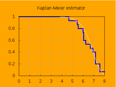
We have plotted in white color the true survival function, which we know, since our sample have been generated by simulation.
Let's now try to estimate parameters a and b from the sample. One of the standard methods is via the maximum likelihood. But in this case we'll use a method based on linear regression. See the following result,
kill(a,b)$
'S(z,a,b) = S(z,a,b);
\[ S\left(z , a , b\right)=e^ {- \left({{z}\over{b}}\right)^{a} } \]
log(lhs(%)) = log(rhs(%));
\[ \log S\left(z , a , b\right)=-\left({{z}\over{b}}\right)^{a} \]
-lhs(%) = -rhs(%);
\[ -\log S\left(z , a , b\right)=\left({{z}\over{b}}\right)^{a} \]
log(lhs(%)) = ev(log(rhs(%)), logexpand = all);
\[ \log \left(-\log S\left(z , a , b\right)\right)=a\,\left(\log z- \log b\right) \]
lhs(%) = expand(rhs(%));
\[ \log \left(-\log S\left(z , a , b\right)\right)=a\,\log z-a\,\log b \]
According to this last result, there is a linear relationship between \(\log z\) and \(\log \left(-\log S\left(z , a , b\right)\right)\). We can estimate parameters \(m=a\) and \(n=-a\,\log b\) by simple linear regression and then obtain estimators for a and b.
We extract from the sample true life times,
x1: subsample(x, lambda([v], second(v)=1),1);
\[ \pmatrix{7.578\cr 4.671\cr 7.163\cr 6.658\cr 6.905\cr 6.248\cr 5.441\cr 6.05\cr 6.045\cr 7.158\cr 7.158\cr 7.566\cr 6.001\cr 5.537 \cr } \]
Estimate the survival time for each observation,
y1: float(matrixmap(hatS,x1));
\[ \pmatrix{0.06667\cr 0.9333\cr 0.2\cr 0.4667\cr 0.4\cr 0.5333\cr 0.8667\cr 0.6\cr 0.6667\cr 0.2667\cr 0.3333\cr 0.1333\cr 0.7333\cr 0.8\cr } \]
Build a table with the two lists, removing those pairs with zero survival probability to avoid problems with logaritms. This task is performed with function subsample defined in package descriptive,
w: subsample(addcol(x1,y1), lambda([v], second(v)#0.0),1,2);
\[ \pmatrix{7.578&0.06667\cr 4.671&0.9333\cr 7.163&0.2\cr 6.658&0.4667 \cr 6.905&0.4\cr 6.248&0.5333\cr 5.441&0.8667\cr 6.05&0.6\cr 6.045& 0.6667\cr 7.158&0.2667\cr 7.158&0.3333\cr 7.566&0.1333\cr 6.001& 0.7333\cr 5.537&0.8\cr } \]
Now we transformate this matrix to obtain pairs of the form \( \left( \log z, \log \left(-\log \hat{S}\left(z\right) \right) \right)\). Function transform_sample, also from package descriptive, is our friend here,
pts: transform_sample(w, [a,b], [log(a),log(-log(b))]) $
\[ \pmatrix{2.025&0.9962\cr 1.541&-2.674\cr 1.969&0.4759\cr 1.896&- 0.2716\cr 1.932&-0.08742\cr 1.832&-0.4642\cr 1.694&-1.944\cr 1.8&- 0.6717\cr 1.799&-0.9027\cr 1.968&0.279\cr 1.968&0.09405\cr 2.024& 0.7006\cr 1.792&-1.171\cr 1.711&-1.5\cr } \]
We are now ready for a least square adjustment,
load (lsquares)$

le: float(lsquares_estimates(pts,
                             [u,v],
                             v=m*u+n,
                             [m,n],
                             initial=[3,3],
                             iprint=[-1,0]));
\[ \left[ \left[ m=7.315 , n=-14.07 \right] \right] \]
Since \(m=a\) and \(n=-a\,\log b\), the estimator for a is
aa: rhs(le[1][1]) ;
\[ 7.315 \]
And for b,
float(solve(−aa*log(b)= rhs(le[1][2])));
\[ \left[ b=6.845 \right] \]
Remember that our sample was obtained by simulation with \(a=10\) and \(b=7\).
© 2017, TecnoStats.