Once you have opened a Maxima session, load package draw:
load("draw") $
To read the documentation on object points, write the following sentence:
describe(points) $
Discrete samples. Points can be entered in two ways: [[x1,y1],[x2,y2],...] or [[x1,x2,...],[y1,y2,...]]:
draw2d(
  key           = "puntitos",
  points(makelist([random(20),random(50)],k,1,10)),
  point_type    = 6,
  point_size    = 2,
  points_joined = true,
  color         = blue,
  key           = "puntazos",
  points(makelist(k,k,1,20),makelist(random(30),k,1,20)),
  file_name     = "puntos",
  terminal      = svg)$
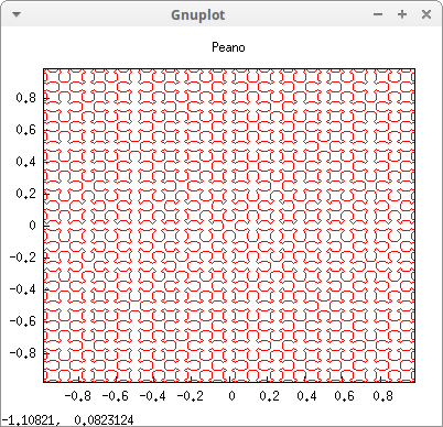
Peano's curve:
load(fractals)$

draw2d(
  point_size    = 0,
  points_joined = true,
  color         = red,
  title         = "Peano",
  points(sierpinskimap(5)) ) $
No comments:
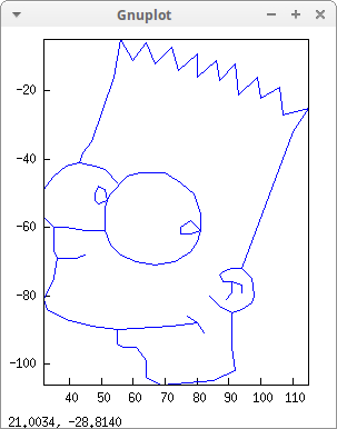
bs:[[64,-104], [64,-99], [61,-95], [57,-95], [55,-94], [55,-90],
    [72,-89], [80,-88], [77,-86], [80,-88], [82,-91], [80,-88],
    [72,-89], [55,-90], [47,-89], [39,-87], [33,-84], [32,-81],
    [35,-75], [36,-69], [42,-69], [45,-68], [42,-69], [36,-69],
    [35,-67], [35,-62], [35,-60], [39,-60], [45,-61], [51,-61],
    [53,-65], [56,-68], [61,-70], [67,-71], [73,-70], [78,-67],
    [80,-64], [81,-61], [78,-58], [75,-60], [75,-62], [78,-62],
    [81,-61], [81,-56], [79,-50], [75,-47], [70,-44], [62,-44],
    [58,-45], [53,-50], [52,-52], [49,-53], [48,-52], [48,-50],
    [49,-48], [51,-49], [52,-52], [51,-54], [51,-57], [51,-61],
    [45,-61], [39,-60], [35,-60], [32,-57], [32,-52], [32,-49],
    [35,-45], [39,-42], [43,-41], [48,-42], [51,-43], [55,-47],
    [51,-43], [48,-42], [43,-41], [44,-38], [47,-35], [54,-16],
    [56,-5], [60,-11], [64,-6], [67,-12], [72,-7], [74,-14],
    [80,-9], [80,-16], [86,-11], [87,-17], [92,-12], [93,-21],
    [99,-16], [100,-22], [106,-19], [107,-27], [115,-25], [110,-32],
    [94,-72], [91,-72], [88,-73], [87,-74], [88,-76], [91,-76],
    [91,-79], [89,-81], [91,-79], [91,-76], [94,-77], [94,-79],
    [94,-77], [91,-76], [88,-76], [87,-74], [88,-73], [91,-72],
    [94,-72], [97,-75], [98,-80], [97,-82], [94,-84], [91,-85],
    [87,-83], [84,-80], [87,-83], [91,-85], [91,-95], [92,-102],
    [85,-105], [69,-106], [64,-104]]$

draw2d(
  point_type    = dot,
  points_joined = true,
  points(bs) )$
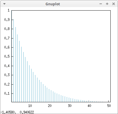
Option points_joined also accepts value impulses:
draw2d(
  points_joined = impulses,
  line_width    = 2,
  color         = light_blue,
  points(makelist(exp(-k/10),k,0,50)) )$
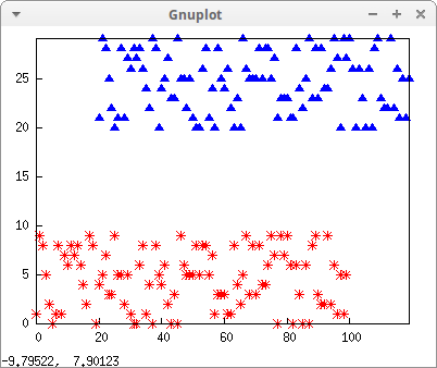
Transforming discrete points stored in an array:
xy: make_array(flonum, 100, 2) $

for i:0 thru 99 do (
  xy[i, 0]: float(i),
  xy[i, 1]: random(10) ) $


draw2d(
   point_type = asterisk,
   point_size = 1.5,
   color      = red,
   points(xy),

   color      = blue,
   transform  = [x+20,y+20,x,y],
   point_type = filled_up_triangle,
   points(xy)) $
Plane transformations:
/* set defaults to avoid writing them many times */
set_draw_defaults(
  points_joined     = true,
  point_type        = dot,
  proportional_axes = 'xy) $

/* builds a grid */
malla(x0,x1,y0,y1) :=
  block([dx, dy, n:21],
    dx: (x1-x0)/n,
    dy: (y1-y0)/n,
    append(
       makelist(
          points(makelist([x0+j*dx, y0+k*dy],
                          k, 1, n)),
          j, 1, n),
       makelist(
          points(makelist([x0+j*dx, y0+k*dy],
                          j, 1, n)),
          k, 1, n)) )$

/* an auxiliary function */
module(x,y) := sqrt(x^2+y^2) $

/* draw a non-transformed grid */
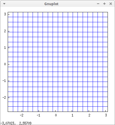
draw2d(
  dimensions = [400,400],
  malla(-%pi,%pi,-%pi,%pi)) $
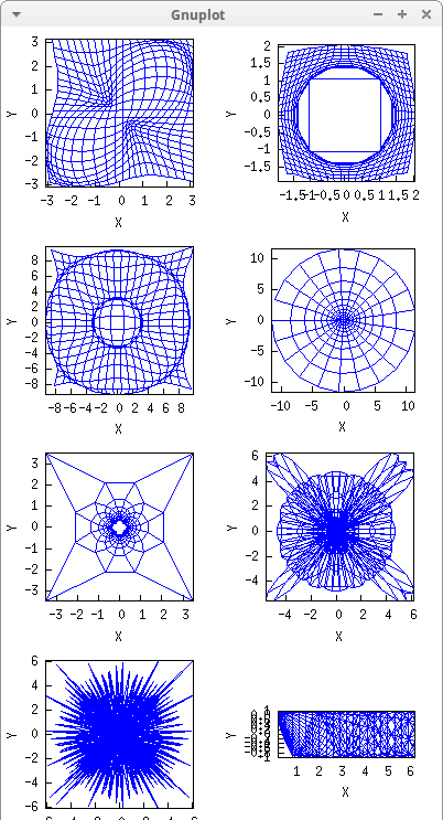
Let's apply some transformations:
tr1 :
  block([k : sin(x)*sin(y)/module(x,y)],
    gr2d(transform = [k*x+x, k*y+y, x, y],
         malla(-%pi,%pi,-%pi,%pi) )) $

tr2 :
  block([k : 1.25/(module(x,y)+0.8)/module(x,y) ],
    gr2d(transform = [k*x+x, k*y+y, x, y],
         malla(-3/2,3/2,-3/2,3/2) )) $

tr3 :
  block([k : sin(module(x,y))/module(x,y) ],
    gr2d(transform = [k*x+x, k*y+y, x, y],
         malla(-3*%pi,3*%pi,-3*%pi,3*%pi) )) $

tr4 :
  gr2d(transform = [realpart(cos(x+y*%i)),
                    imagpart(cos(x+y*%i)),
                    x, y],
       malla(-%pi, %pi, -%pi, %pi) ) $

tr5 :
  gr2d(transform = [realpart(1/conjugate(x+y*%i)),
                    imagpart(1/conjugate(x+y*%i)),
                    x, y],
       malla(-3, 3, -3, 3) ) $

tr6 :
  block([k : sin(module(x,y))],
    gr2d(transform = [k*x, k*y, x, y],
         malla(-2*%pi, 2*%pi, -2*%pi, 2*%pi) )) $

tr7 :
  block([k : sin(x*y)],
    gr2d(transform = [k*x, k*y, x, y],
         malla(-2*%pi, 2*%pi, -2*%pi, 2*%pi) )) $

tr8 :
  gr2d(transform = [y, cos(x*y), x, y],
       malla(0, %pi, 0, 2*%pi ) ) $

draw(
  dimensions = [400,750],
  columns    = 2,
  tr1, tr2, tr3, tr4, tr5, tr6, tr7, tr8 ) $
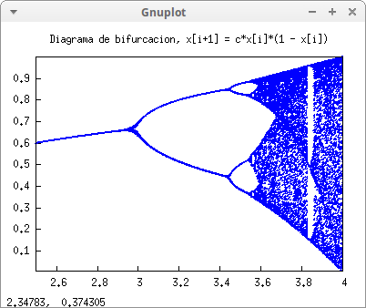
Bifurcation diagram:
pts:[]$

for c:2.5 while c <= 4.0 step 0.002 do
  (x: 0.75,
   for k:1 thru 50 do x: c * x * (1-x),
   for k:1 thru 50 do
     (x: c * x * (1-x),
      pts: cons([c,x], pts))) $

draw2d(
  title      = "Diagrama de bifurcacion, x[i+1] = c*x[i]*(1 - x[i])",
  point_type = filled_circle,
  point_size = 0.5,
  points(pts)) $
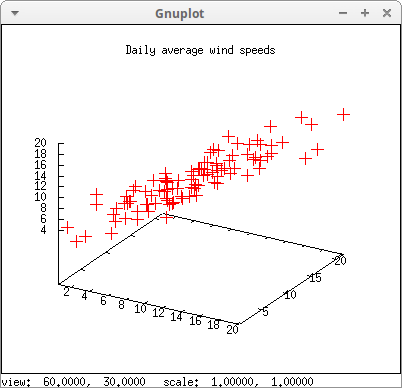
File wind.data, which is included in the Maxima, contains daily average wind speeds at 5 meteorological stations in the Republic of Ireland (This is part of a data set taken at 12 meteorological stations. The original file is freely downloadable from the StatLib Data Repository and its analysis is discused in Haslett, J., Raftery, A. E. (1989) Space-time Modelling with Long-memory Dependence: Assessing Ireland's Wind Power Resource, with Discussion. Applied Statistics 38, 1-50).
In this example, data corresponding to stations number 1, 2 and 3 are represented coordinates in the 3d space
s2 : read_matrix (file_search ("wind.data"))$

draw3d(
  title      = "Daily average wind speeds",
  point_size = 2,
  color      = red,
  points(submatrix (s2, 4, 5)) )$
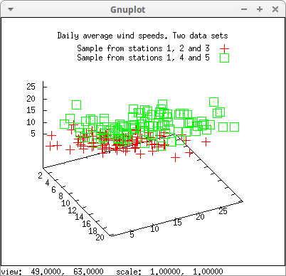
Following with the previous example, now data corresponding to stations 1, 4 and 5, are also plotted:
draw3d(
  title      = "Daily average wind speeds. Two data sets",
  point_size = 2,
  color      = red,
  key        = "Sample from stations 1, 2 and 3",
  points(submatrix (s2, 4, 5)),
  point_type = 4,
  color      = green,
  key        = "Sample from stations 1, 4 and 5",
  points(submatrix (s2, 2, 3)) )$
Coordinates can be given in two different list-formats:
xx: [1,2,3,4,5]$
yy: [4,5,7,1,2]$
zz: [3,2,1,9,4]$
xyz: [[10,15,12],[11,13,16],[16,10,11],[15,15,15]]$

draw3d(
  point_size    = 2,
  point_type    = filled_square,
  color         = blue,
  points(xx,yy,zz),

  point_type    = circle,
  color         = green,
  points_joined = true,
  points(xyz)) $

Discrete data can be also joined by lines. This is an example of Brownian motion in 3d:
block([history:[[0,0,0]], lst, pos],

   for k:1 thru 1000 do
      (lst: copylist(last(history)),
       pos: random(3)+1,
       lst[pos]: lst[pos] + random(2)*2-1,
       history: endcons(lst, history) ),

   draw3d(
     title         = "Brownian motion in 3D",
     terminal      = eps,
     dimensions    = 100*[10,10],
     point_size    = 0,
     points_joined = true,
     points(history) )  )$

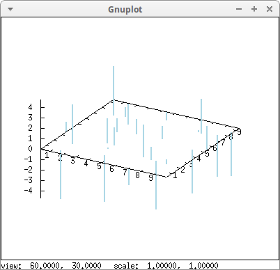
Impulses in 3D:
draw3d(
  points_joined = impulses,
  line_width    = 2,
  color         = "light-blue",
  xyplane       = 0,
  points(makelist([random(10.0),random(10.0),random(10.0)-5],k,0,25)) )$
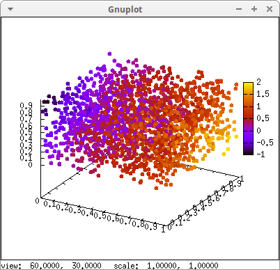
Discrete points can be colored with respect to their (x, y, z) coordinates:
m: makelist([random(1.0),random(1.0),random(1.0)],k,1,2000)$

draw3d(
  point_type = filled_circle,
  enhanced3d = [u+v-w,u,v,w], /* variable names are arbitrary */
  points(m) ) $
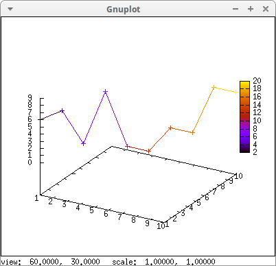
Since points are declared in a certain order, their colors can be defined according to an ordering index, which we call j in this example:
m: makelist([k, k, random(10)],k,1,10)$

draw3d(
 enhanced3d    = [sin(j), j],
 line_width    = 2,
 point_type    = circle,
 points_joined = true,
 colorbox      = false,
 points(m)) $

We can create a list of scalars to be associated to each point. Pay attention to the simple quote:
scalars : makelist(k*2, k, 1, 10)$

m: makelist([k, k, random(10)],k,1,10)$

draw3d(
 enhanced3d    = ['part(scalars, k), k],
 points_joined = true,
 points(m) ) $
Translated points in 3D:
xyz: make_array(fixnum, 10, 3) $
for i:0 thru 9 do (
   xyz[i, 0]: random(10),
   xyz[i, 1]: random(10),
   xyz[i, 2]: random(10) ) $

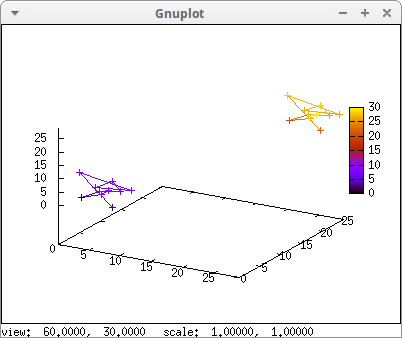
draw3d(
   enhanced3d    = true,
   points_joined = true,
   points(xyz),
   transform     = [x+20,y+20,z+20,x,y,z],
   points(xyz)) $
The benzene molecule in the wxt terminal. For higher quality molecule graphics, give the VTK interface a try:
atomo(x,y,z):=
  parametric_surface(x+cos('a)*cos('b),
                     y+cos('b)*sin('a),
                     z+sin('b), 'a,0,2*%pi,'b,-%pi/2,%pi/2) $

block([s,v,numer:true],
       s: 5*sqrt(3)/2,
       v: 5*sqrt(3),
       draw3d(
         /* Preamble */
         title   = "Benzene C6H6",
         axis_3d = false,
         surface_hide   = true,
         xu_grid        = 10,
         yv_grid        = 5,
         user_preamble  = "set size ratio 1",
         zrange = [-5,5],
         terminal = wxt,

         /* links */
         point_size    = 0,
         color         = black,
         points_joined = true,
         line_width    = 3,
         points([[0,10,0],[0,5,0],[s,5/2,0],[v,5,0]]),
         points([[v,-5,0],[s,-5/2,0],[0,-5,0],[0,-10,0]]),
         points([[-v,5,0],[-s,5/2,0],[-s,-5/2,0],[-v,-5,0]]),
         points([[0,5,1/2],[-s,5/2,1/2]]),
         points([[0,5,-1/2],[-s,5/2,-1/2]]),
         points([[-s,-5/2,1/2],[0,-5,1/2]]),
         points([[-s,-5/2,-1/2],[0,-5,-1/2]]),
         points([[s,5/2,1/2],[s,-5/2,1/2]]),
         points([[s,5/2,-1/2],[s,-5/2,-1/2]]),

         /* Hydrogen */
         color         = green,
         atomo(0,10,0),
         atomo(0,-10,0),
         atomo(v,5,0),
         atomo(v,-5,0),
         atomo(-v,5,0),
         atomo(-v,-5,0),
         color = black,
         label(["H",0,10,1.5],["H",0,-10,1.5],
               ["H",v,5,1.5],["H",v,-5,1.5],
               ["H",-v,5,1.5],["H",-v,-5,1.5]),

         /* Carbon */
         color         = blue,
         atomo(0,5,0),
         atomo(0,-5,0),
         atomo(s,5/2,0),
         atomo(s,-5/2,0),
         atomo(-s,5/2,0),
         atomo(-s,-5/2,0),
         color = black,
         label(["C",0,5,1.5],["C",0,-5,1.5],
               ["C",s,5/2,1.5],["C",s,-5/2,1.5],
               ["C",-s,5/2,1.5],["C",-s,-5/2,1.5]) ))$

© 2011-2016, TecnoStats.