Standardization means to subtract to each element the sample mean and then dividing by the standard deviation. We need to load package descriptive before calling function standardize.
load("descriptive")$
standardize([1,2,3,4,5,6,7,8,9]);
[−2√3√5,−3322√5,−√3√5,−√32√5,0,√32√5,√3√5,3322√5,2√3√5]
When the argument is a matrix, rows are interpreted as individual characteristics and each element is standardized with respect to the mean and standard deviation of its column,
m : matrix([3,3,7,8],[4,6,5,0],[7,6,5,4],[7,2,8,3],[0,6,2,6]) $
standardize(m);
(−6√105√87−8√5√198√105√5319√5√46−√105√877√5√19−2√105√53−21√5√4614√105√877√5√19−2√105√53−1√5√4614√105√87−13√5√1913√105√53−6√5√46−21√105√877√5√19−17√105√539√5√46)
Given a multivariate sample, we can extract subsamples according to certain conditions.
n : matrix([A,3,7,8],[B,6,5,0],[A,6,5,4],[A,2,8,3],[B,6,2,6]);

/* function 'takeA' will be applied to all rows,
   extracting those beginning with letter A */
takeA(v) := is(first(v)='A)$
subsample(n, takeA);
(A378A654A283)
Following with this example, we can select rows with more conditions, at the time we remove or reorder the columns.
takeA5(v) := is(first(v)='A and second(v) < 5)$
subsample(n, takeA5, 2, 4, 3);
(387238)
Now, we keep those individuals whose sum of components is greater than certain value.
subsample(m, lambda([z], apply("+", z) > 20));
(33787654)
While function subsample filters records (rows) in multivariate samples, function tranform_sample can be used to transform, remove and create variables (columns).
transform_sample needs three arguments: the sample matrix, a list with the names of the variables, and a list indicating how to build the new matrix.
Given a matrix, we want to build a new matrix with the following conditions:
d : matrix([3,3,7,8],[4,6,5,0],[7,6,5,4],[7,2,8,3],[1,6,2,6]) $

transform_sample(
    d,
    [x1, x2, x3, x4],
    [log(x1), x2*x3, x1, makelist(1,k,length(d))]);
(log32131log43041log73071log7167101211)
This time we want to standardize the fourth column of the original matrix. Pay attention to the single quote operator applied to the list of transforming expressions, this is necessary to avoid the execution of standardize before calling tranform_sample.
transform_sample(
    d,
    [x1, x2, x3, x4],
    '[x1, standardize(x4), x1^2]);
(3192√4694−212√46167−12√46497−3√4649192√461)
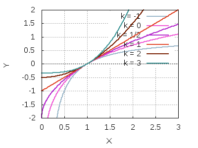
Box-Cox transformations help to approximate data to a Gaussian distribution. This property is necessary for applying a large set of statistical procedures. They are defined as bc(x,k,m)={log(x+m)if k=0(x+m)k−1kotherwise where k is the power to which data will be raised, and m is a constant used to avoid negative values. We plot Box-Cox transformations for different values of parameter k,
bc(x,k,m) :=
    if k=0
        then log(x+m)
        else ((x+m)^k-1) / k $

draw2d(
    yrange     = [-2,2],
    line_width = 2,
    grid       = true,
    xaxis      = true,
    yaxis      = true,
    map(lambda([z], [color = random_color(),
                     key   = string('k = z),
                     explicit( bc(x,z,0), x, 0, 3)]),
        [-1, 0, 1/2, 1, 2, 3]) ) $

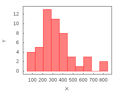
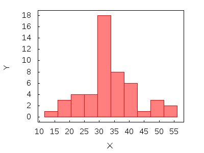
Here is a worked example to show how to apply this procedure,
/* the sample and its histogram */
m: [299.9,195.0,155.8,478.7,396.7,640.7,457.8,46.59,298.5,109.3,
    397.5,91.28,278.5,815.6,842.2,252.8,351.4,370.4,250.8,572.3,
    414.6,428.7,94.81,372.7,321.8,221.0,222.5,320.0,233.1,290.9,
    263.2,319.6,480.9,274.6,164.9,656.6,362.0,168.8,401.3,292.6,
    269.0,270.6,442.5,277.2,284.8,300.8,251.1,320.9,674.0,177.0] $
histogram(m, fill_density = 0.5) $

/* since it seems to be a certain level of positive skewness,
   we apply a Box-Cox transformation  */
m2: bc(m,1/2,0)$
histogram(m2, fill_density = 0.5) $

This was an example of a Box-Cox transformation applied to a sample list. Let's now transform columns of a matrix,
d : matrix([3,3,7,8],[4,6,5,0],[7,6,5,4],[7,2,8,3],[1,6,2,6]);

transform_sample(
    d,
    [x1, x2, x3, x4],
    '[bc(x3, 6, 0), bc(x1, 0, 1)]);
(19608log42604log52604log8873812log8212log2)
Again, do not forget the simple quote.
© 2011-2016, TecnoStats.