ML estimators in normal populations

Acronym ML stands for maximum likelihood.

ML estimators are calculated in such a way that they maximize the likelihood of n independent observations. That is, if $f(x_i; \theta_1, \ldots, \theta_p)$ is the value of the density function for the i-th observation, which depends on parameters $\theta_1, \ldots, \theta_p$, the function to be maximized is $$L(\theta_1, \ldots, \theta_p; x_1, \ldots, x_n) = \prod_{i=1}^n f(x_i; \theta_1, \ldots, \theta_p).$$ The set of numbers $\hat{\theta}_1, \ldots, \hat{\theta}_p$, such that they maximize $L$, are the so called maximum likelihood estimators.

First, we load package distrib,

load("distrib")$

Given a normal, or gaussian, population with unknown parameters $\mu$ and $\sigma$, once we have an independent sample of size n, $(x_1, x_2, \ldots, x_n)$, our likelihood function takes the form

L: product(pdf_normal(x[i],mu,sigma), i, 1, n);

$$\prod_{i=1}^{n}{{{e^ {- {{\left(x_{i}-\mu\right)^2}\over{2\,\sigma^ 2}} }}\over{\sqrt{2}\,\sqrt{\pi}\,\sigma}}}$$

Taking the logarithm of the above expression, we get the loglikelihood function,

logL: ev(log(L), logexpand=all);

$$\sum_{i=1}^{n}{\left(-\log \sigma-{{\left(x_{i}-\mu\right)^2}\over{ 2\,\sigma^2}}-{{\log \pi}\over{2}}-{{\log 2}\over{2}}\right)}$$

As we want to maximize the likelihood, or equivalently the loglikelihood, we need to equal to zero the partial derivatives of the loglikelihood with respect to $\mu$ and $\sigma$. The derivative with respect to $\mu$ is

logLmu: ev(diff(logL, mu), simpsum=true);

$${{\sum_{i=1}^{n}{x_{i}}-\mu\,n}\over{\sigma^2}}$$

Equating to zero and isolating $\mu$ yields

hatmu: solve(logLmu, mu);

$$\left[ \mu={{\sum_{i=1}^{n}{x_{i}}}\over{n}} \right]$$

Which we recognize as the sample mean, so that our result can be summarized as $\hat{\mu}=\bar{x}$.

We repeat a similar procedure for $\sigma^2$,

logLsi: ev(diff(logL, sigma), simpsum=true) $
hatsi: solve(logLsi, sigma^2);

$$\left[ \sigma^2={{\sum_{i=1}^{n}{\left(x_{i}-\mu\right)^2}}\over{n }} \right]$$

Which is the sample variance, so that $\hat{\sigma}^2=s^2$.

The expression for the variance can be written only in terms of the sample values,

subst(hatmu, hatsi);

$$\left[ \sigma^2={{\sum_{i=1}^{n}{\left(x_{i}-{{\sum_{i=1}^{n}{x_{i} }}\over{n}}\right)^2}}\over{n}} \right]$$

Let us now proceed with the numerical part of this session. Instead of taking our sample from a real world population, we can make a simulation calling function random_normal from package distrib. Let $n=50$ be the sample size, $\mu=50$, and $\sigma=2.5$,

(n: 50, mu: 50, sigma: 2.5) $
fpprintprec: 4 $
x: random_normal(mu, sigma, n) ;

$$\left[ 53.21 , 50.45 , 52.16 , 51.37 , 44.37 , 52.65 , 50.92 , 51.25 , 52.18 , 48.49 , \\ 52.49 , 46.19 , 47.32 , 47.73 , 50.58 , 48.6 , 49.21 , 52.32 , 49.95 , 48.7 , \\ 55.38 , 51.36 , 48.3 , 49.34 , 52.6 , 48.8 , 47.52 , 44.53 , 49.25 , 44.47 , \\ 48.58 , 48.33 , 48.39 , 49.36 , 43.98 , 53.73 , 51.93 , 51.76 , 46.22 , 53.61 , \\ 51.2 , 50.16 , 54.3 , 46.86 , 56.86 , 49.21 , 50.75 , 45.22 , 53.87 , 48.85 \right]$$

In order to calculate the sample mean and variance, we need to load the descriptive package. We also include the sample standard deviation,

load("descriptive") $
ml: [mean(x), var(x), std(x)];

$$\left[ 49.9 , 8.529 , 2.92 \right]$$

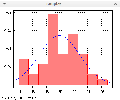
As a result, $\hat{\mu}=49.9$, and $\hat{\sigma}=2.92$. Remember that our sample was artificially drawn from a normal population with parametrrs $\mu=50$, and $\sigma=2.5$. Also remember that the ML estimator of the variance is a biased estimator.

With help of function histogram, also implemented in package descriptive, we can show a graphical representation of the sample together with the estimated gaussian probability density,

[m, s]: [ml[1], ml[3]] $
draw2d(
    grid       = true, 
    dimensions = [400,300],
    histogram_description(
        x,
        nclasses     = 9,
        frequency    = density,
        fill_density = 0.5),
    explicit(pdf_normal(z,m,s), z, m - 3*s, m + 3* s) ) $

© 2017, TecnoStats.