This section shows how to make animations with the draw package, both on a window or animated gif file.
Repeated calls to draw creates an animated window:
/* fine tune this variable according to your computer */
delay: 50000$

for d:0.1 thru 1 step 0.1 do
    block([dummy:1],
        while dummy < delay do dummy: dummy+1,
        draw2d(explicit(x^d,x,0,1)) ) $

We can repeat the animation a fixed number of times (five, in this example):
for k:1 thru 5 do
    begin([delay: 50000, dummy],
        for d:0.1 thru 1 step 0.1 do
            (dummy:1,
             while dummy < delay do dummy: dummy+1,
             draw2d(explicit(x^d,x,0,1))) )  $
It is possible to set global option terminal to animated_gif to save the animation in gif format. In this case, the delay is controlled by option delay and the name of the file by file_name. You always need to call directly function draw:
kill(all)$

draw(
  terminal   = animated_gif,
  delay      = 40,
  file_name  = "gifanim",
  dimensions = [400, 400],
  makelist(gr2d(explicit(x^(0.1*k),x,0,1)),k,10)) $

In some systems, animated gifs don't work because gnuplot was compiled without this type of terminal. In these cases, it is necessary to call external programs (imagemagick is an option here). With the following code you can get the same result as in the previous example. Firts, a set of png's are saved in your working folder and then function convert of the imagemagick collection builds the animated gif:
for k:1 thru 10 do
  draw2d(terminal   = png,
         file_name  = concat("ga",add_zeroes(k)),
         dimensions = [400, 400],
         explicit(x^(0.1*k),x,0,1)) $

/* This was tested in Linux: */
system("convert -delay 40 *.png gifanim.gif")$
Terminal animated_gif of the draw package does not handle multiplots. In this case, proceed as in this example calling an external program.
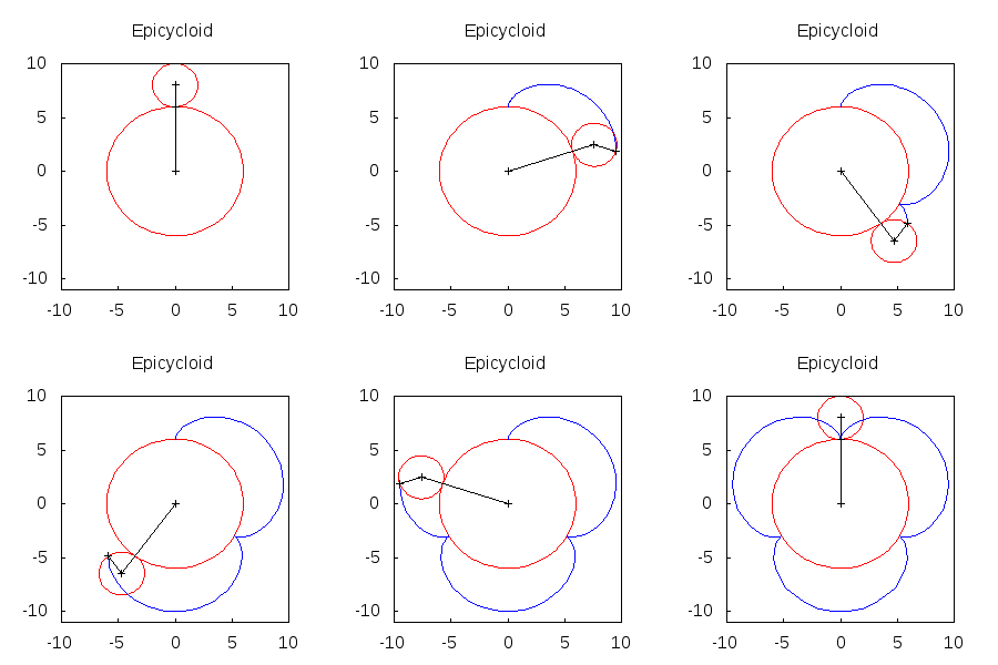
An animated epicycloid:
/*
This function returns a list of gr2d objects, which
are the consecutive frames to be packed in the animated
gif file.
   R = Radius of great circumference
   r = radius of small circumference
   n = number of frames
*/
epicycloids(R,r,n):=
  block([x,y,a,end_point,ang,epis:[]],
    x: (R+r)*sin(a)-r*sin(a*(1+R/r)),
    y: (R+r)*cos(a)-r*cos(a*(1+R/r)),
    for k:0 thru n do
       (ang: float(k * 2*%pi/n),
        end_point: subst(a=ang,[x,y]),
        epis: cons(gr2d(
                     dimensions = [300,300],
                     title      = "Epicycloid",
                     xrange     = [-10,10],
                     yrange     = [-11,10],
                     nticks     = 80,
                     color      = red,
                     parametric(R*cos(u),
                                R*sin(u),
                                u,0,2*%pi),
                     parametric((R+r)*sin(ang)+r*cos(u),
                                (R+r)*cos(ang)+r*sin(u),
                                u,0,2*%pi),
                     color = blue,
                     parametric(x,y,a,0,ang),
                     color      = black,
                     point_size = 1,
                     points_joined = true,
                     points([[0,0],(R+r)*[sin(ang),cos(ang)],end_point])),
                   epis )),
    reverse(epis) )$

apply(draw, append([terminal=animated_gif, delay=20],
                    epicycloids(6,2,20))) $

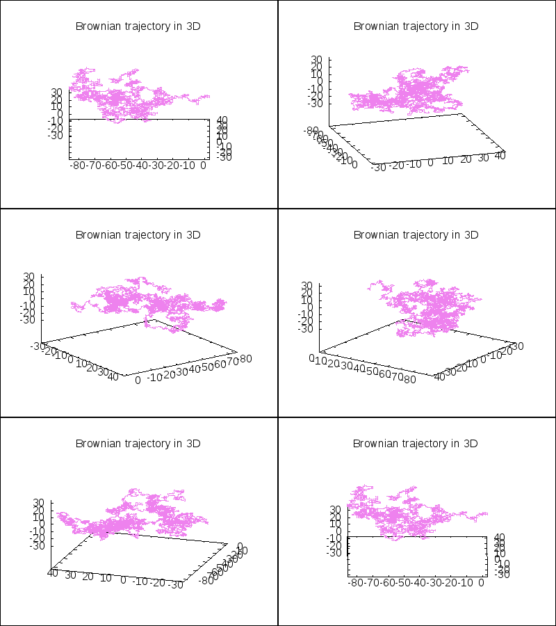
A 3D Brownian trajectory viewed with different angles:
brown_simulation:
  block([history:[[0,0,0]], lst, pos],
   for k:1 thru 10000 do
      (lst: copylist(last(history)),
       pos: random(3)+1,
       lst[pos]: lst[pos] + random(2)*2-1,
       history: endcons(lst, history) ),
   history) $

apply(draw, append([terminal=animated_gif, delay=20, file_name="brownian"],
                    makelist(gr3d(title         = "Brownian trajectory in 3D",
                                  view          = [60, k*18],
                                  point_size    = 0,
                                  points_joined = true,
                                  color         = violet,
                                  points(brown_simulation) ),
                             k,0,20)))$

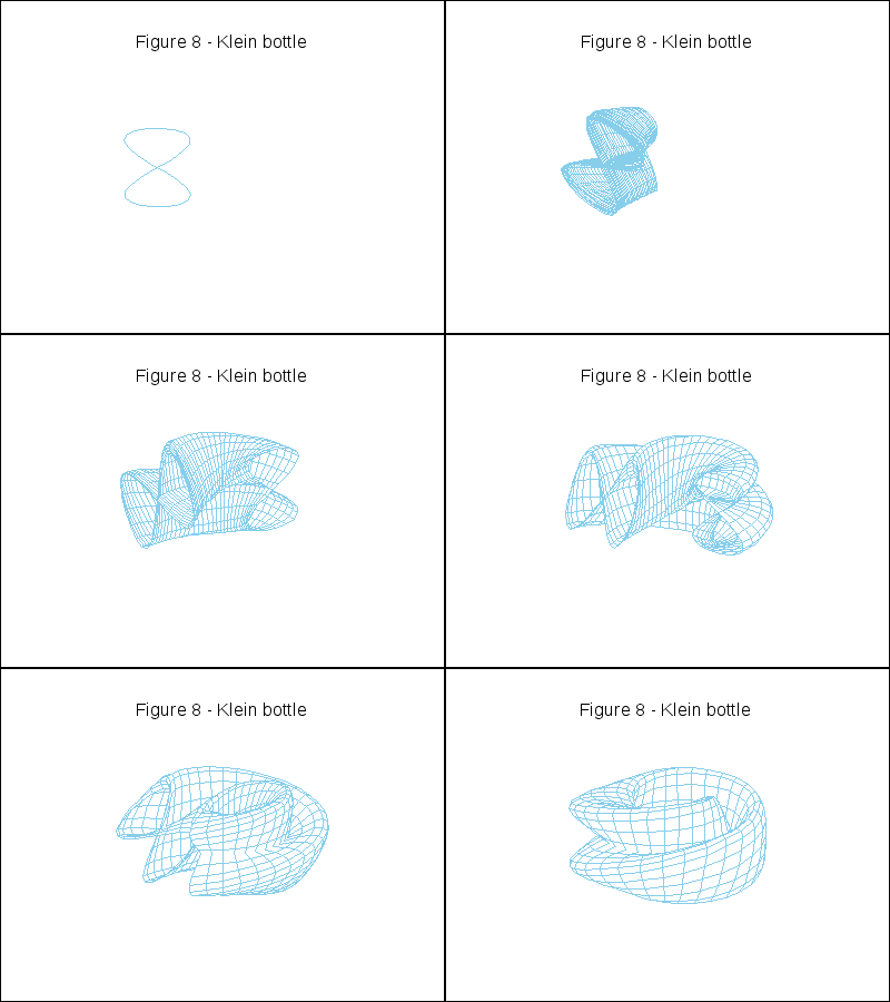
A topological example. Construction of the figure-8 Klein Bottle:
apply(draw,
      append([terminal=animated_gif, delay=30],
             makelist(
               gr3d(title        = "Figure 8 - Klein bottle",
                    view         = [60,10 * k],
                    xrange       = [-3.4,3.4],
                    yrange       = [-3.4,3.4],
                    zrange       = [-1.4,1.4],
                    axis_3d      = false,
                    surface_hide = true,
                    color        = skyblue,
                    parametric_surface(
                       (2+cos(u/2)*sin(v)-sin(u/2)*sin(2*v))*cos(u),
                       (2+cos(u/2)*sin(v)-sin(u/2)*sin(2*v))*sin(u),
                       sin(u/2)*sin(v) + cos(u/2)*sin(2*v),
                       u, -%pi, 10*k*%pi/180-%pi, v, 0, 2*%pi) ),
               k,0,36)))$

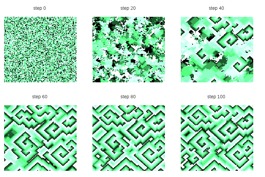
Cyclic cellular automaton simulation: starting from an initial random state, this dynamical model based on local rules exhibits self organized patterns. See http://en.wikipedia.org/wiki/Cyclic_cellular_automaton for a reference. Function ca_cyclic_von_neumann is defined in file cyclic.lisp. :
(/* CA package loading */
 load("path/cyclic.lisp"),

 /* A 100 x 100 cellular space */
 nr: 100,
 nc: 100,

 /* cellular automaton parameters */
 n_states: 10,
 threshold: 1,
 n_iterations: 100,

 /* initial random state */
 ini: apply(matrix, makelist(makelist(random(n_states),k,1,nc),j,1,nr)),

 /* simulation process */
 im: ca_cyclic_von_neumann(ini,n_states,threshold,n_iterations),

 /* global drawing options */
 global_options:
   [terminal    = animated_gif,
    delay       = 20,
    file_name   = "cyclic_ca",
    dimensions   = [300,300]],

 frames:
   makelist(gr2d(title       = concat("step ",k),
                 colorbox    = false,
                 axis_top    = false,
                 axis_right  = false,
                 axis_left   = false,
                 axis_bottom = false,
                 xtics       = none,
                 ytics       = none,
                 ztics       = none,
                 palette     = [3,21,-10],
                 image(im[k+1],0,0,1,1)),
             k,0,n_iterations),

 /* this part may take a while! */
 apply(draw, append(global_options, frames)) )$

© 2011-2016, TecnoStats.