
Once you have opened a Maxima session, load package draw:
load("draw") $
To read the documentation on object explicit, write the following sentence:
describe(explicit) $
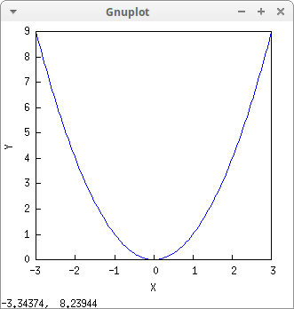
Function draw2d describes a scene in two dimensions. In this case, an explicit function in the screen terminal:
draw2d(explicit(u^2,u,-3,3))$
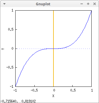
Another explicit function. In this case, axes are drawn with different styles:
draw2d(explicit(x^3,x,-1,1),
       xaxis       = true,
       xaxis_color = blue,
       yaxis       = true,
       yaxis_width = 2,
       yaxis_type  = solid,
       yaxis_color = "#f3b507") $
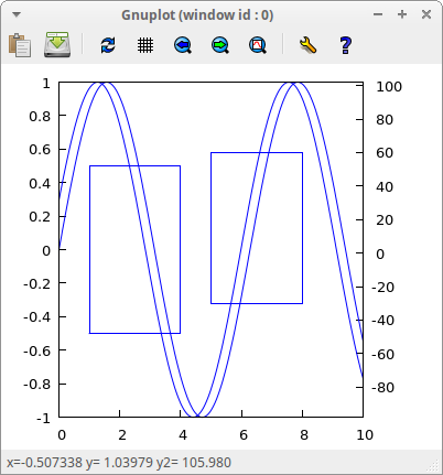
With the secondary y-axis, it is possible to plot functions with respect to two scales of ordinates. The secondary y-axis is drawn on the right. All 2d objects are sensible to local graphics option yaxis_secondary. Other possible options related to the secondary y-axis are: yrange_secondary, ytics_secondary, ytics_axis_secondary and ytics_rotate_secondary:
draw2d(
   terminal        = wxt,
   transparent     = true,
   explicit(sin(x),x,0,10),
   rectangle([1,-1/2],[4,1/2]),
   yaxis_secondary = true,
   ytics_secondary = true,
   explicit(100*sin(x+0.3)+2,x,0,10),
   rectangle([5,-30],[8,60])) $
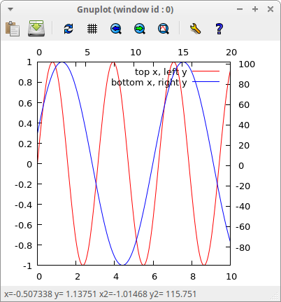
The secondary x-axis is drawn on top of the scene. All 2d objects are sensible to local graphics option xaxis_secondary. Other possible options related to the secondary x-axis are: xrange_secondary, xtics_secondary, xtics_axis_secondary and xtics_rotate_secondary:
draw2d(
   /* activate both secondary axes */
   xtics_secondary = auto,
   ytics_secondary = auto,

   /* red curve is plotted against secondary x-axis and primary y-axis */
   xaxis_secondary = true,
   color           = red,
   key             = "top x, left y",
   explicit(sin(x),x,0,20),

   /* blue curve is plotted against primary x-axis and secondary y-axis */
   xaxis_secondary = false,
   yaxis_secondary = true,
   color           = blue,
   key             = "bottom x, right y",
   explicit(100*sin(x+0.3)+2,x,0,10),
   terminal        = wxt) $
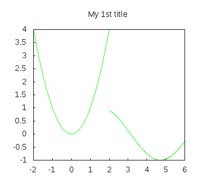
Piecewise function. This time, the result is saved in a png file. Options terminal and title, since they are global, can be written in any place:
draw2d(
  color     = green,
  explicit(u^2,u,-2,2),
  explicit(sin(z),z,2,6),
  terminal  = png,
  title     = "My 1st title") $
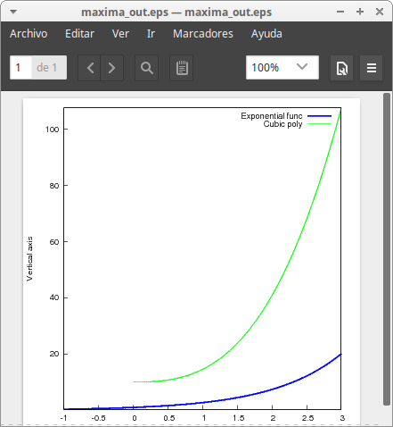
Two different explicit functions. We want the result in an eps file:
draw2d(
  terminal   = eps_color,
  dimensions = 100*[10,10],
  key        = "Exponential func",
  color      = blue,
  line_width = 4,
  explicit(exp(x),x,-1,3),
  line_width = 2,
  color      = "#00ff00",   /* green, in hexadecimal */
  key        = "Cubic poly",
  explicit(%pi*x^3+sqrt(2)*x^2+10,x,0,3),
  xlabel     = "Horizontal axis",
  ylabel     = "Vertical axis") $
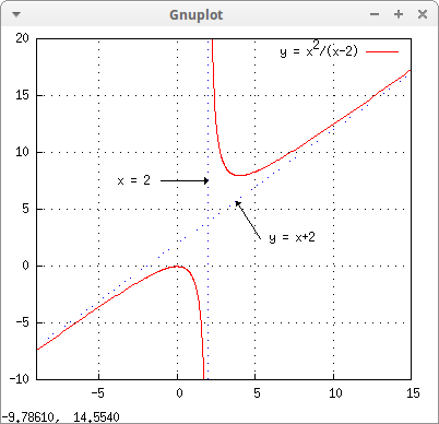
A rational function and its asymptotes:
draw2d(
  /* the rational function */
  grid   = true,
  key    = "y = x^2/(x-2)",
  yrange = [-10,20],
  color  = red,
  explicit(x^2/(x-2),x,-9,15),

  /* asymptotes */
  key       = "",
  line_type = dots,
  color     = blue,
  explicit(x+2,x,-9,15),
  nticks    = 70,
  parametric(2,t,t,-10,20),

  /* labels and arrows */
  head_length = 0.3,
  color       = black,
  line_type   = solid,
  vector([5.35,2.45],[-1.53,3.25]),
  vector([-1,7.5],[3,0]),
  label_alignment = left,
  label(["y = x+2",6,2.5]),
  label_alignment = right,
  label(["x = 2",-1.7,7.5])) $
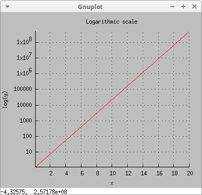
Logarithmic scales:
draw2d(
  background_color = gray,
  logy             = true,
  xlabel           = "x",
  ylabel           = "log(y)",
  color            = red,
  explicit(exp(x),x,0.1,20),
  axis_top         = false,
  axis_right       = false,
  grid             = true,
  title            = "Logarithmic scale") $
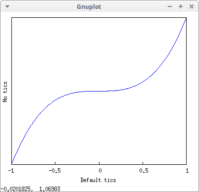
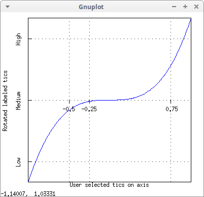
The following examples show how to place tics on axes:
draw2d(
  xlabel = "Default tics",
  ylabel = "No tics",
  ytics  = 'none,
  explicit(x^3,x,-1,1))  $
draw2d(
  xlabel = "Start-increment-end",
  ylabel = "Tics intervals 0.25",
  xtics  = [-3/4,1/8,3/4],
  ytics  = 1/4,
  explicit(x^3,x,-1,1) ) $

draw2d(
  xlabel     = "User selected tics on axis",
  ylabel     = "Rotated labeled tics",
  xtics      = {-1/2,-1/4,3/4}, /* set of numbers */
  xtics_axis = true,            /* plot tics on x-axis */
  ytics      = {["High",0.75],["Medium",0],["Low",-0.75]},
  ytics_rotate = true,
  grid       = true,
  explicit(x^3,x,-1,1)  ) $
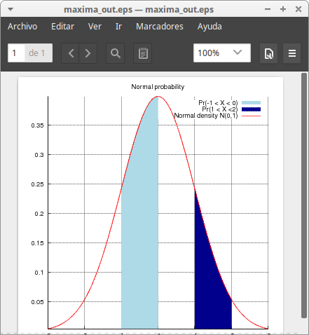
Filled functions. By default, graphics option filled_func is set to false. When it is set to true, the region bounded by the function and the bottom of the graphics region is filled with color fill_color:
load(distrib)$

draw2d(
  terminal    = eps_color,
  dimensions  = 100*[10,10],
  title       = "Normal probability",
  grid        = true,
  axis_top    = false,
  axis_right  = false,
  filled_func = true,
  fill_color  = "light-blue",
  key         = "Pr(-1 < X < 0)",
  explicit(pdf_normal(x,0,1),x,-1,0),
  key         = "Pr(1 < X <2)",
  fill_color  = "dark-blue",
  explicit(pdf_normal(x,0,1),x,1,2),
  filled_func = false,
  color       = red,
  key         = "Normal density N(0,1)",
  explicit(pdf_normal(x,0,1),x,-3,3)  ) $
It is also possible to fill the region bounded by two explicit functions. You only need to set graphics option filled_func to the expression of the second function. Take into account that the variable used in this expression must be the same used in the explicit object. In this example, note that when you call explicit the second time, filled_func= sin(x) is still active:
draw2d(
  fill_color  = grey,
  filled_func = sin(x),
  explicit(-sin(x),x,0,%pi),
  fill_color  = cyan,
  explicit(-sin(x),x,%pi,2*%pi)) $

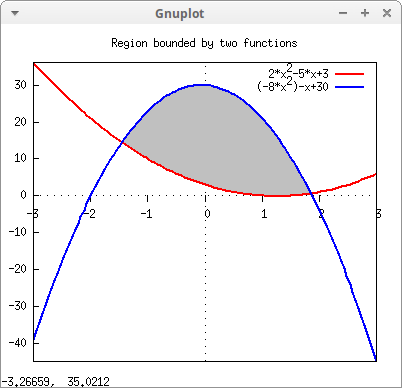
A more elaborated example:
f1: 2*x^2-5*x+3$
f2: -8*x^2-x+30$

[x1,x2]: map('rhs, solve(f1=f2)) $

draw2d(title       = "Region bounded by two functions",
       fill_color  = grey,
       filled_func = f2,
       explicit(f1,x,x1,x2),
       filled_func = false,
       xaxis       = true,
       xtics_axis  = true,
       yaxis       = true,
       line_width  = 2,
       key         = string(f1),
       color       = red,
       explicit(f1,x,-3,3),
       key         = string(f2),
       color       = blue,
       explicit(f2,x,-3,3) ) $
Translating and rotating a parabola:
th : %pi/6 $

draw2d(
  xrange            = [-2,5],
  yrange            = [-1,6],
  proportional_axes = 'xy,

  explicit(x^2,x,-1,1),
  transform         = [cos(th)*x - sin(th)*y + 3,
                       sin(th)*x + cos(th)*y + 3, x, y],
  color             = red,
  explicit(x^2,x,-1,1) )$

Comparing logarithmic and non logarithmic scales in 3D:
draw(
  dimensions = [400,600],
  gr3d(
    title = "Z: non-logarithmic scale",
    color = red,
    explicit(exp(u^2+v^2),u,0,5,v,0,5)),
  gr3d(title = "Z: logarithmic scale",
    logz  = true,
    color = red,
    explicit(exp(u^2+v^2),u,0,5,v,0,5)))$

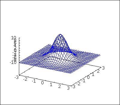
An explicit function in GIF format:
draw3d(
  terminal = gif,
  explicit(20*exp(-x^2-y^2)-10,x,-3,3,y,-3,3)) $
Another explicit function. In this case, axis and xy-grid are drawn. Note that the user_preamble option is used to draw the grid at z=0 level:
draw3d(
  explicit(x^2+y^2,x,-1,1,y,-1,1),
  xaxis_width=2, xaxis_color=orange, xaxis_type=solid, xaxis=true,
  yaxis_width=2, yaxis_color=orange, yaxis_type=solid, yaxis=true,
  zaxis_width=2, zaxis_color=blue,   zaxis_type=solid, zaxis=true,
  grid          = true,
  user_preamble = "set xyplane at 0" ) $

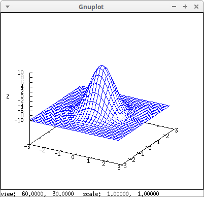
Hidding surfaces:
draw3d(
  surface_hide = true,
  explicit(20*exp(-x^2-y^2)-10,x,-3,3,y,-3,3)) $
Two explicit functions:
draw3d(
  key          = "Gauss",
  explicit(20*exp(-x^2-y^2)-10,x,-3,3,y,-3,3),
  yv_grid      = 10,
  color        = red,
  key          = "Plane",
  explicit(x+y,x,-5,5,y,-5,5),
  surface_hide = true)$

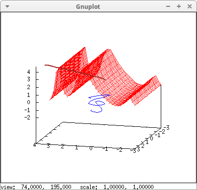
An explicit surface and two parametric curves:
draw3d(
  color = red,
  explicit(exp(sin(x)+cos(x^2)),x,-3,3,y,-3,3),

  color = blue,
  parametric(cos(5*u)^2,sin(7*u),u-2,u,0,2),

  color = brown,
  line_width = 2,
  parametric(t^2,sin(t),2+t,t,0,2) ) $
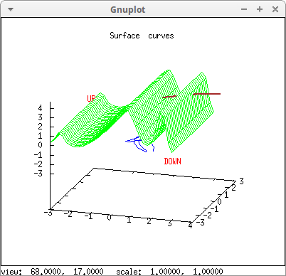
The same as before, but with hidden surfaces and labels:
draw3d(
  color = green,
  explicit(exp(sin(x)+cos(x^2)),x,-3,3,y,-3,3),

  color = blue,
  parametric(cos(5*u)^2,sin(7*u),u-2,u,0,2),

  color = brown,
  line_width = 2,
  parametric(t^2,sin(t),2+t,t,0,2),
  surface_hide = true,
  title = "Surface & curves",
  color = red,
  label(["UP",-2,0,3]),
  label(["DOWN",2,0,-3]) ) $
A composition with 3d objects:
draw3d(
  surface_hide = true,
  xlabel       = "x",
  ylabel       = "y",
  zlabel       = "z",

  color        = "light-blue",
  parametric_surface(u**2-v**2,2*u*v,u, u,-3,3,v,-3,3),

  color   = coral,
  xu_grid = 20,
  yv_grid = 10,
  explicit(10+exp(0.3*sin(x^2/10)+0.2*cos(x^3/5)),x,-10,10,y,-10,10),

  color      = black,
  line_width = 2,
  nticks     = 40,
  parametric(15*cos(r),10*sin(r),2*r-10,r,0,4*%pi) ) $
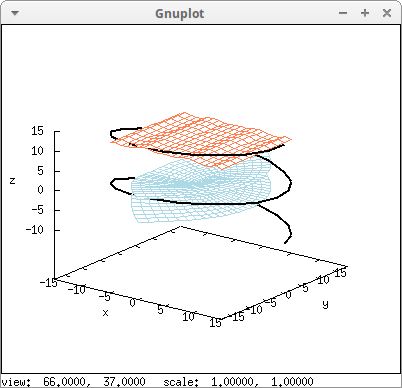
Reflected explicit surface:
surf: explicit(20*exp(-x^2-y^2)-10,x,-3,3,y,-3,3) $

draw3d(
  color     = "#a02c00",
  surf,
  transform = [x,y,-z,x,y,z],
  color     = blue,
  surf )$

Global graphics option enhanced3d sets Gnuplot's pm3d mode:
draw3d(
  enhanced3d   = true,
  explicit(20*exp(-x^2-y^2)-10,x,-3,3,y,-3,3)) $
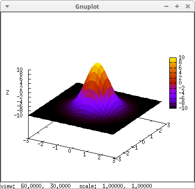
The same as before, but without the colorbox:
draw3d(
  enhanced3d   = true,
  colorbox     = false,
  explicit(20*exp(-x^2-y^2)-10,x,-3,3,y,-3,3)) $

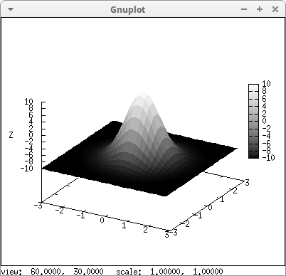
Changing the color palette to gray:
draw3d(
  enhanced3d   = true,
  palette      = gray,
  explicit(20*exp(-x^2-y^2)-10,x,-3,3,y,-3,3)) $
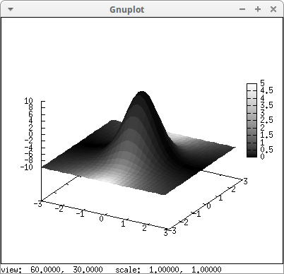
An explicit object is defined in terms of the (x, y) coordinates, and we can define color numbers in terms of x and y:
draw3d(
  palette    = gray,
  enhanced3d = [y^(10/7)/(x^2+1),x,y],
  explicit(20*exp(-x^2-y^2)-10,x,-3,3,y,-3,3))$
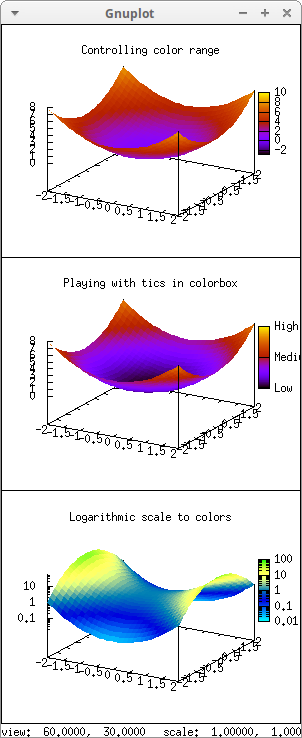
There are some global graphic options for controlling the range and the tics in the colorbox. This example also demonstrates how to build a multiplot:
example1:
  gr3d (title          = "Controlling color range",
        enhanced3d     = true,
        color          = green,
        cbrange        = [-3,10],
        explicit(x^2+y^2, x,-2,2,y,-2,2)) $

example2:
  gr3d (title          = "Playing with tics in colorbox",
        enhanced3d     = true,
        color          = green,
        cbtics         = {["High",10],["Medium",05],["Low",0]},
        cbrange = [0, 10],
        explicit(x^2+y^2, x,-2,2,y,-2,2)) $

example3:
  gr3d (title      = "Logarithmic scale to colors",
        enhanced3d = true,
        color      = green,
        logcb      = true,
        logz       = true,
        palette    = [-15,24,-9],
        explicit(exp(x^2-y^2), x,-2,2,y,-2,2)) $

draw(
  dimensions = [300,700],
  example1, example2, example3) $
Setting another color palette. Write ? palette to learn how it works:
draw3d(
  enhanced3d   = true,
  palette      = [25,-10,35],
  explicit(20*exp(-x^2-y^2)-10,x,-3,3,y,-3,3)) $

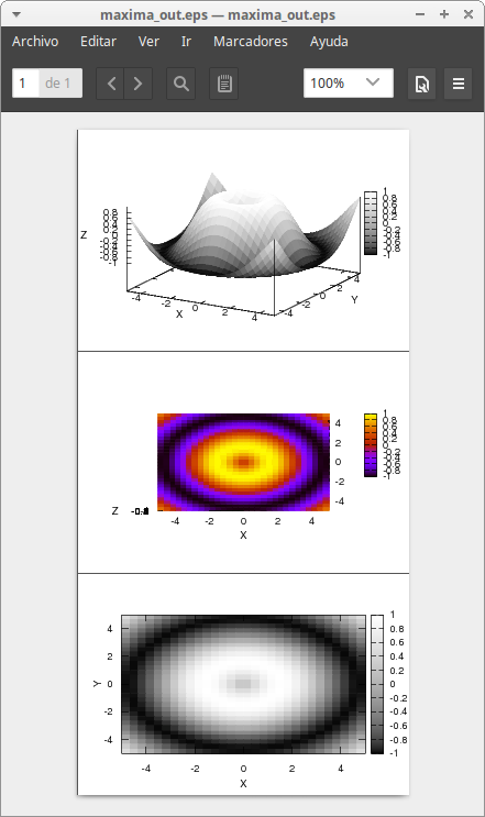
Setting another color palette. Write ? palette to learn how it works:
scene1: gr3d(
          surface_hide = true,
          enhanced3d   = true,
          palette      = gray,
          explicit(sin(sqrt(x^2+y^2)),x,-5,5,y,-5,5))$

/* A density plot, looking the surface from above */
scene2: gr3d(
          surface_hide   = true,
          enhanced3d     = true,
          view           = [0, 360],
          explicit(sin(sqrt(x^2+y^2)),x,-5,5,y,-5,5))$

/* Gnuplot experts would prefere to make use of option 'user_preamble' */
scene3: gr3d(
          surface_hide  = true,
          enhanced3d    = true,
          palette       = gray,
          user_preamble = "set pm3d map",
          explicit(sin(sqrt(x^2+y^2)),x,-5,5,y,-5,5))$

/* Plot all together in a Postscript file */
draw(
  terminal   = eps_color,
  dimensions = 100*[8, 16],
  scene1,
  scene2,
  scene3) $
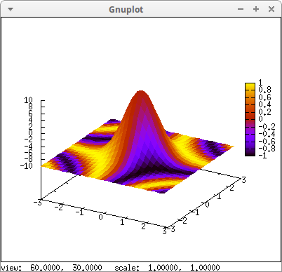
By default, when graphics option enhanced3d is set to true, colors depend on the z-values, but when this option is set to an expression, colors depend on the result of this expression and on the actual value of option palette. This is useful for drawing four dimensional plots, where the fourth dimension is given by the color. Note that the expression passed to enhanced3d depends on variables x and y, as in the explicit object below:
draw3d(
  enhanced3d   = sin(x*y),
  explicit(20*exp(-x^2-y^2)-10, x ,-3, 3, y, -3, 3)) $
Another example with two surfaces. Option palette is global, and it can be used only once, since multiple palettes are not allowed in the same plot. :
draw3d(
  surface_hide = true,
  palette      = gray,
  xu_grid      = 50,
  yv_grid      = 50,

  enhanced3d   = true,  /* equivalent to  enhanced3d = 5*sin(x*y) */
  explicit(5*sin(x*y), x, -5, 5, y, -5, 5),

  enhanced3d   = 5 * sin(v*u),
  explicit(u^2+v^2+10, u, -5, 5, v, -5, 5)) $

In this case, enhanced3d is used to draw a shadowed surface. (Thanks to Richard Hennessy for this example.):
f(x,y,z):=z-20*exp(-x^2-y^2)-10 $
fn1(x,y):=20*exp(-x^2-y^2)-10 $

grad:[diff(f(x,y,z),x),diff(f(x,y,z),y),diff(f(x,y,z),z)] /
          sqrt(diff(f(x,y,z),x)^2+diff(f(x,y,z),y)^2+diff(f(x,y,z),z)) $
light:[-1/sqrt(3),-1/sqrt(3),1/sqrt(3)] $
dotprod(x,y,z):=grad.light $

draw3d(
  palette      = [4,5,6],
  xu_grid      = 100,
  yv_grid      = 100,
  colorbox     = false,
  enhanced3d   = dotprod(x,y,fn1(x,y)),
  explicit(fn1(x,y), x ,-3, 3, y, -3, 3)) $

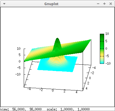
The same two explicit surfaces as above, but with enhanced colors:
draw3d(
  enhanced3d   = true,
  palette      = [15,-8,-5],
  explicit(20*exp(-x^2-y^2)-10,x,-3,3,y,-3,3),
  explicit(x+y,x,-5,5,y,-5,5)) $
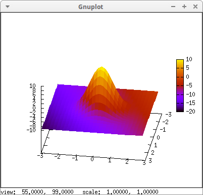
We can define number colors with respect to the three coordinates of the points:
draw3d(
  enhanced3d = [z-x+2*y,x,y,z],
  explicit(20*exp(-x^2-y^2)-10,x,-3,3,y,-3,3))$
Playing with random colors:
load(distrib)$

draw3d(
  palette    = [2,25,-21],
  enhanced3d = ['random_normal(z/5,1),x,y,z],
  explicit(20*exp(-x^2-y^2)-10,x,-3,3,y,-3,3))$

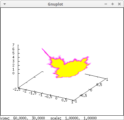
Projecting the Mandelbrot set on a paraboloid:
load(fractals)$

draw3d(
  xu_grid    = 100,
  yv_grid    = 100,
  colorbox   = false,
  palette    = [2,25,-21],
  enhanced3d = ['mandelbrot_set(x,y),x,y],
  explicit(x^2+y^2,x,-2.5,1,y,-1,1))$
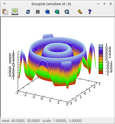
User defined palettes are allowed. Assign option palette a list of colors. Surface points with lowest value, according to enhanced3d, will be assigned the first color in the list, and with heighest value the last color, the rest are interpolated:
draw3d(
  terminal   = wxt,
  xu_grid    = 100,
  yv_grid    = 100,
  palette    = ["#ff0000", green, orange, "#450cd2", light_blue],
  enhanced3d = [z,x,y,z], /* point with coordinates (x,y,z) has */
                          /* level z */
  explicit(sin(x^2+y^2),x,-3,3,y,-3,3) )$
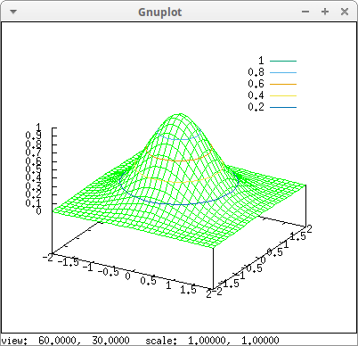
It is possible to fix the number of isolines setting option contour_levels to a positive integer number. The actual number of levels can be adjusted to give simple labels, as in this example:
draw3d(
  surface_hide   = true,
  color          = green,
  explicit(exp(-x^2-y^2),x,-2,2,y,-2,2),
  contour        = surface,
  contour_levels = 3) $
Declare increments to isolines setting contour_levels to a list of the form [init, incr, end]:
draw3d(
  surface_hide   = true,
  color          = green,
  explicit(exp(-x^2-y^2),x,-2,2,y,-2,2),
  contour        = surface,
  contour_levels = [0.1,0.1,1]) $
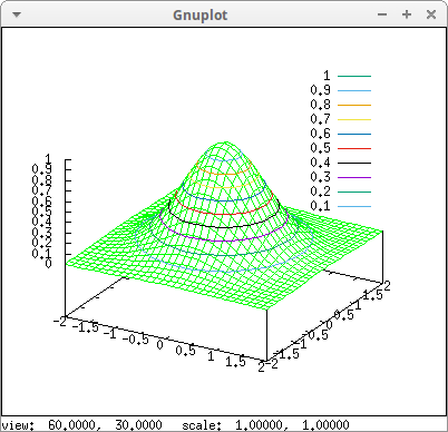
It is also possible to select a certain number of fixed levels setting contour_levels to a set of numbers:
draw3d(
  surface_hide   = true,
  color          = green,
  explicit(exp(-x^2-y^2),x,-2,2,y,-2,2),
  contour        = surface,
  contour_levels = {0.1,0.7,0.8}) $
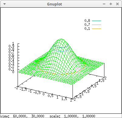
In this case, contour lines are added in the xy-plane:
draw3d(
  color          = green,
  explicit(20*exp(-x^2-y^2)-10,x,0,2,y,-3,3),
  yv_grid        = 10,
  color          = red,
  explicit(x+y,x,0,2,y,-5,5),
  contour_levels = 15,
  contour        = base,
  surface_hide   = true)  $

More contours:
draw3d(
  color          = green,
  explicit(20*exp(-x^2-y^2)-10,x,0,2,y,-3,3),
  contour_levels = 15,
  contour        = both,
  surface_hide   = true) $
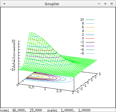
Contours projected on the plane:
draw3d(
  terminal       = eps_color,
  title          = "Contours projected on the plane",
  explicit(20*exp(-x^2-y^2)-10,x,0,2,y,-3,3),
  contour_levels = 15,
  contour        = map,
  surface_hide   = true) $
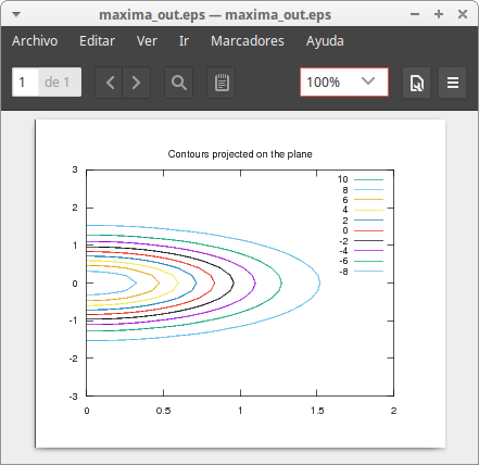
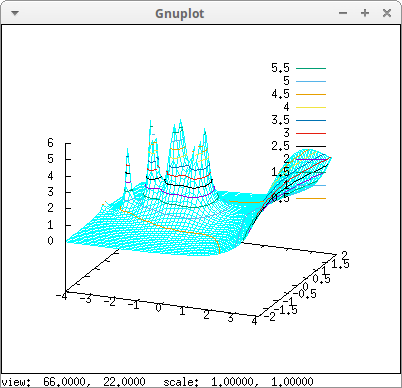
Absolute value of the gamma function:
gamma2(x,y):=
   block([re,im,g:gamma(x+%i*y)],
     re:realpart(g),
     im:imagpart(g),
     sqrt(re^2+im^2))$

draw3d(
  zrange=[0,6],
  xu_grid        = 50,
  yv_grid        = 50,
  surface_hide   = true,
  contour        = surface,
  contour_levels = [0,0.5,6], /* from 0 to 6 in steps of 0.5 */
  color          = cyan,
  explicit(gamma2(x,y),x,-4,4,y,-2,2)) $
Absolute value of the polynomic function z3+1 with enhanced color and contours:
z3(x,y):= abs((x+y*%i)^3+1)$

draw3d(
  contour    = both,
  enhanced3d = true,
  explicit(z3(x,y),x,-10,10,y,-10,10)) $

© 2011-2016, TecnoStats.