
Once you have opened a Maxima session, load package worldmap:
load("worldmap") $
To read the documentation on object geomap, write the following sentence:
describe(geomap) $
This section shows how to plot cartographic maps with the draw package. The graphic object to be used is geomap, where the argument is a list of integer indices (beginning with 0) of the global Lisp array boundaries_array.
Some of the examples below can take a while to be rendered.
Let's draw Barbados:
draw2d(geomap(Barbados))$
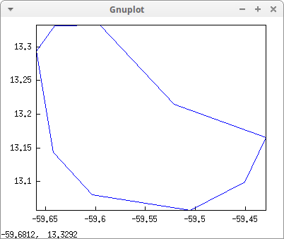
This is the value of variable Barbados as defined in package worldmap:
Barbados;
[[2139]]
All country boundaries are defined in an special array of arrays called boundaries_array, and number 2139 tells us that the coast of Barbados is the 2139th element of boundaries_array:
boundaries_array[2139];
{Lisp Array: #(-59.505001 13.05694
               -59.450569 13.09944
               -59.429169 13.165
               -59.521118 13.21444
               -59.59584 13.33194
               -59.641109 13.33139
               -59.65918 13.29305
               -59.642231 13.14361
               -59.603611 13.08
               -59.505001 13.05694)}
Which is a set of ten coordinates pairs defining the polygonal line that represents the coast of Barbados.
Package worldmap contains coast lines and boundaries coordinates in (longitude, latitude) format in region [-180,180]×[-90,90]. When the package is loaded, global variable boundaries_array is set to an array of length 2801, each element being another array containing the coordinates of a boundary:
arrayinfo(boundaries_array);
[declared,1,[2800]]
The map of Antigua and Barbuda:
draw2d(geomap(Antigua_and_Barbuda))$
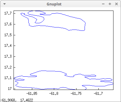
This country needs two arrays, one for each island:
Antigua_and_Barbuda;
[[2082],[2088]]
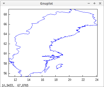
Sweden, with its continental lines and islands:
draw2d(geomap(Sweden))$
Sweden;
[[1473,1474,1475,1542,1543,1547,1596,1614,1612,1565,1513,1481,1446,1430,1390],[1557],[1593],[1581]]
The structure of Sweden is a bit more complex. Arrays 1473 thru 1390 define the coast line and/or the borders with other countries, while arrays 1557, 1593, and 1581 are the islands Orust, Öland, and Gotland, respectively.
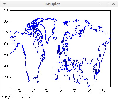
Let's now plot boundaries from 1000 to 2000:
draw2d(geomap(makelist(k,k,1000,2000))) $
The complete map:
draw2d(geomap(makelist(k,k,0,2800))) $
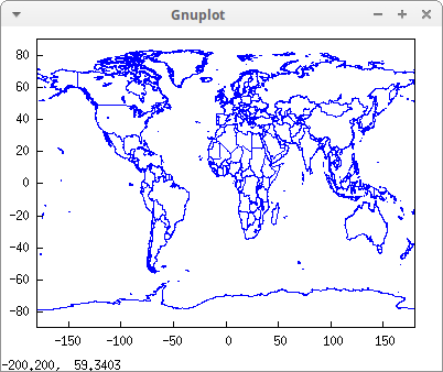
Let's plot some countries and continents:
c1: gr2d(geomap([Canada,United_States,Mexico,Cuba]))$
c2: gr2d(geomap([Africa]))$
c3: gr2d(geomap([Oceania,China,Japan]))$
c4: gr2d(geomap([France,Portugal,Spain,Morocco,Western_Sahara]))$
draw(
  dimensions = [600,500],
  terminal   = svg,
  columns    = 2,
  c1,c2,c3,c4) $
There are in worldmap some utilities of interest, especially for defining new geographical objects. Sicily (south Italy) is not defined in worldmap, but we know that it is in the rectangular region defined by vertices 10.4E 41.5N and 20.7E 35.4N (just tell Maxima to plot Italy and move the mouse around). Now call function region_boundaries to know which vertices are within this region and plot them:
z: region_boundaries(10.4,41.5,20.7,35.4);
[1846,1863,1864,1881,1888,1894]
draw2d(geomap(z))$
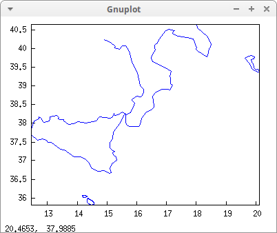
With this output, you don't know how to define Sicily as a Maxima variable, but you can call function numbered_boundaries, also defined in worldmap, to see the numbers of the polygonal segments:
numbered_boundaries(z)$
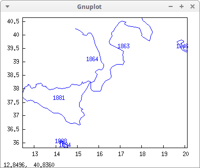
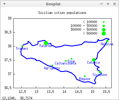
We know now that Sicily is formed by boundary number 1881. Let's make use of it:
Sicily: [1881]$
/* cities coordinates and populations from wikipedia */
labs: label(["Agrigento",13.583,37.317 - 0.1],
            ["Caltanisseta",14.067,37.4833 - 0.1],
            ["Catania",15.066,37.517 - 0.1],
            ["Enna",14.276,37.5633 - 0.1],
            ["Messina",15.55,38.183 - 0.1],
            ["Palermo",13.367,38.117 - 0.1],
            ["Ragusa",14.75,36.933 - 0.1],
            ["Siracusa",15.283,37.083 - 0.1],
            ["Trapani",12.517,38.017 - 0.1] )$
pop1: points([[13.583,37.317],    /* Agrigento */
              [14.067,37.4833],   /* Caltanisseta */
              [14.276,37.5633],   /* Enna */
              [14.75,36.933],     /* Ragusa */
              [12.517,38.017]])$  /* Trapani */
pop2: points([[15.55,38.183],     /* Messina */
              [15.283,37.083]])$  /* Siracusa */
pop3: points([[15.066,37.517]])$  /* Catania */
pop4: points([[13.367,38.117]])$  /* Palermo */
draw2d(yrange     = [36.5,39],
       xrange     = [12.2,15.7],
       title      = "Sicilian cities populations",
       line_width = 3,
       geomap(Sicily),
       point_type = filled_circle,
       color = green,
       key = "       < 100000", point_size = 1, pop1,
       key = "100000 - 300000", point_size = 1.5, pop2,
       key = "300000 - 500000", point_size = 2, pop3,
       key = "       > 500000", point_size = 2.5, pop4,
       color = blue,
       labs )$
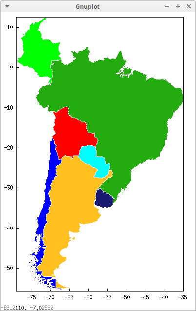
With function make_poly_country in package worldmap it is possible to build polygonal objects from country names, so that they can be filled with different colours. The return value of make_poly_country is a list of polygons, since some countries need more than just one polygonal because of the islands. A simple example follows:
draw2d(
  dimensions = [400,600],
  color      = white, /* white country borders */

  fill_color = red,             make_poly_country(Bolivia),
  fill_color = cyan,            make_poly_country(Paraguay),
  fill_color = green,           make_poly_country(Colombia),
  fill_color = blue,            make_poly_country(Chile),
  fill_color = "#23ab0f",       make_poly_country(Brazil),
  fill_color = goldenrod,       make_poly_country(Argentina),
  fill_color = "midnight-blue", make_poly_country(Uruguay) ) $
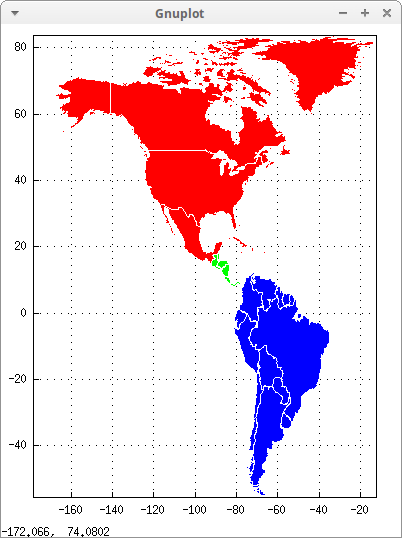
There is also make_poly_continent to build polygonal objects from continent names or lists of countries:
draw2d(
  dimensions = [400,500],
  grid       = true,
  color      = white, /* white country borders */
  fill_color = red,    make_poly_continent(North_America),
  fill_color = green,  make_poly_continent(Central_America),
  fill_color = blue,   make_poly_continent(South_America) )$
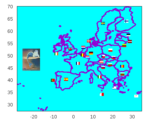
Variable European_Union is defined in worldmap. You can download the flags and the mermaid from here:
load(picture)$

draw2d(
  terminal   = png,
  dimensions = [500,400],
  /* background */
  border     = false,
  fill_color = cyan,
  rectangle([-28.80,27.53],[34.79,70.26]),
  /* boundaries */
  line_width = 3,
  color      = "dark-violet",
  geomap(European_Union),
  /* flags */
  image(read_xpm("path/austria.xpm"),13.3,46.9,2,1.2),
  image(read_xpm("path/belgium.xpm"),3.66,49.77,2,1.2),
  image(read_xpm("path/bulgaria.xpm"),24,42,2,1.2),
  image(read_xpm("path/cyprus.xpm"),31,33,2,1.2),
  image(read_xpm("path/czech_republic.xpm"),14.18,49.15,2,1.2),
  image(read_xpm("path/denmark.xpm"),6.86,55.46,2,1.2),
  image(read_xpm("path/estonia.xpm"),27.02,58,2,1.2),
  image(read_xpm("path/finland.xpm"),26.03,63.5,2,1.2),
  image(read_xpm("path/france.xpm"),1.3,46.32,2,1.2),
  image(read_xpm("path/germany.xpm"),8,50.5,2,1.2),
  image(read_xpm("path/greece.xpm"),19.86,36.37,2,1.2),
  image(read_xpm("path/hungary.xpm"),17.65,45.79,2,1.2),
  image(read_xpm("path/ireland.xpm"),-9.69,50.24,2,1.2),
  image(read_xpm("path/italy.xpm"),12.39,40.82,2,1.2),
  image(read_xpm("path/latvia.xpm"),27.71,55.22,2,1.2),
  image(read_xpm("path/lithuania.xpm"),24.89,53.59,2,1.2),
  image(read_xpm("path/luxembourg.xpm"),6.14,48.90,2,1.2),
  image(read_xpm("path/malta.xpm"),13.43,33.69,2,1.2),
  image(read_xpm("path/netherlands.xpm"),4.01,52.88,2,1.2),
  image(read_xpm("path/poland.xpm"),17.86,51.73,2,1.2),
  image(read_xpm("path/portugal.xpm"),-11.56,39.48,2,1.2),
  image(read_xpm("path/romania.xpm"),23.85,45.18,2,1.2),
  image(read_xpm("path/slovakia.xpm"),19.37,48.72,2,1.2),
  image(read_xpm("path/slovenia.xpm"),14.16,44.65,2,1.2),
  image(read_xpm("path/spain.xpm"),-4.79,39.82,2,1.2),
  image(read_xpm("path/sweden.xpm"),14.05,62.63,2,1.2),
  image(read_xpm("path/united_kingdom.xpm"),-2.61,52.11,2,1.2),
  /* the mermaid */
  image(read_xpm("path/sirena.xpm"),-26,44,9,9)  )$
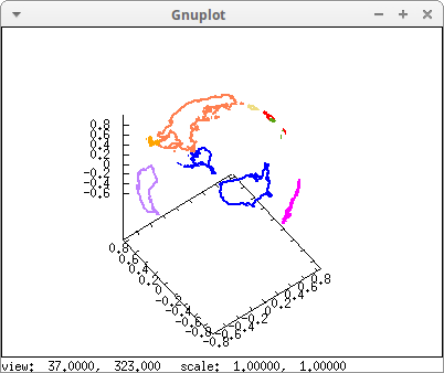
In 3D, maps are projected on the unit sphere (center (0,0,0) and radius 1):
draw3d(
  line_width        = 2,
  proportional_axes = xyz,
  color = blue,              geomap(United_States),
  color = red,               geomap(Spain),
  color = "light-goldenrod", geomap(Germany),
  color = coral,             geomap(Russia),
  color = "#58a30f",         geomap(Portugal),
  color = magenta,           geomap(Brazil),
  color = orange,            geomap(Japan),
  color = purple,            geomap(Australia) )$
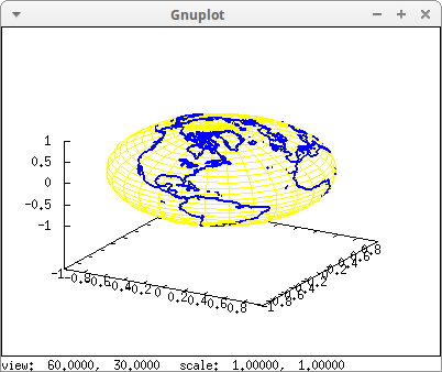
World coastlines and islands projected on the sphere. Variable World_coastlines is defined in package worldmap:
c:%pi/180$

draw3d(
  surface_hide = true,
  color        = yellow,
  parametric_surface(
       cos(phi*c)*cos(theta*c),
       cos(phi*c)*sin(theta*c),
       sin(phi*c),
       theta,-180,180,
       phi,-90,90),
  color      = blue,
  line_width = 2,
  geomap(World_coastlines))$
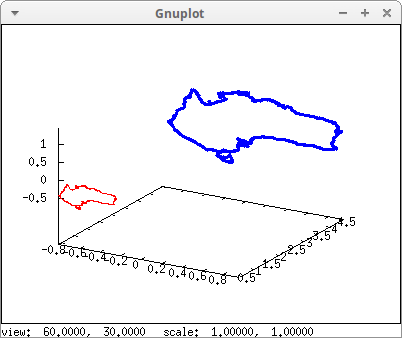
Australia projected on two different spheres:
draw3d(
  color      = red,
  geomap(Australia), /* projected on unit sphere */
  color      = blue,
  line_width = 3,
  geomap([Australia],
         [spherical_projection,2,2,2,3]))$
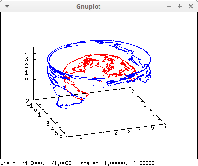
Cylindrical and spherical projections:
draw3d(
  color = red,
  geomap([America_coastlines,Eurasia_coastlines],
         [spherical_projection,2,2,2,3]),
  color = blue,
  geomap([America_coastlines,Eurasia_coastlines],
         [cylindrical_projection,2,2,2,3,4])) $
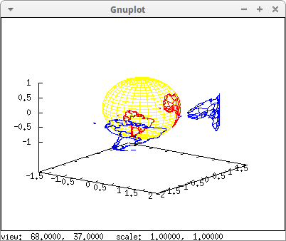
Another example of cylindrical and spherical projections. The sphere is also plotted:
draw3d(
  surface_hide = true,
  view         = [60, 131],
  color        = yellow,
  parametric_surface(
       cos(phi)*cos(theta),
       cos(phi)*sin(theta),
       sin(phi),
       theta,-%pi,%pi,
       phi,-%pi/2,%pi/2),
  color = red,
  geomap([South_America,Africa,Australia],
         [spherical_projection,0,0,0,1]),
  color = blue,
  geomap([South_America,Africa,Australia],
         [cylindrical_projection,0,0,0,1,2]))$
Conic projection:
a:90$
r:1$
[cx,cy,cz]:[0,0,0]$
c: float(%pi/180)$
h:r/sin((a/2) * c)$
R:r/cos((a/2) * c)$
m: sqrt(h^2+R^2)$

draw3d(
  proportional_axes = xyz,
  color = yellow,
  parametric_surface(
        cx+R*cos(theta)*t,
        cy+R*sin(theta)*t,
        cz+(1-t)*h,theta,-%pi,%pi,t,0,1),
  parametric_surface(
        cx+R*cos(theta)*t,
        cy+R*sin(theta)*t,
        cz-(1-t)*h,theta,-%pi,%pi,t,0,1),
  color = black,
  geomap([America_coastlines,Africa_coastlines],
         [conic_projection,cx,cy,cz,r,a]))$
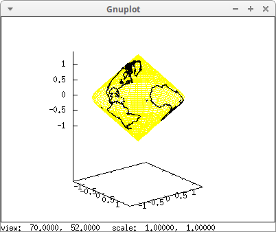
Array boundaries_array does not contain all countries and islands in the world. If we want to add more boundaries, we can proceed as follows.
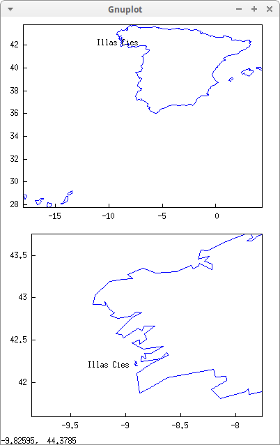
The Cíes Islands are in Galicia, in the northwest of Spain. They are not included in boundaries_array and we want to plot them. First, we see how many arrays are already in boundaries_array:
arrayinfo(boundaries_array);
[declared,1,[2800]]
This means that the last element has index 2800, let's see it
boundaries_array[2800];
{Lisp Array: #(-180.0 -90.0 180.0 -90.0 179.99998 -78.301682)}
Now, we want to add two islands:
b1: make_array(flonum,24)$

( b1[0]: -8.91463, b1[1]: 42.25134,
  b1[2]: -8.90167, b1[3]: 42.24200,
  b1[4]: -8.90073, b1[5]: 42.23100,
  b1[6]: -8.89558, b1[7]: 42.22732,
  b1[8]: -8.90159, b1[9]: 42.22522,
  b1[10]: -8.89935, b1[11]: 42.21708,
  b1[12]: -8.91429, b1[13]: 42.21162,
  b1[14]: -8.91652, b1[15]: 42.21727,
  b1[16]: -8.90622, b1[17]: 42.22458,
  b1[18]: -8.90794, b1[19]: 42.23863,
  b1[20]: -8.91815, b1[21]: 42.25070,
  b1[22]: -8.91463, b1[23]: 42.25134 )$
and
b2: make_array(flonum,10)$

( b2[0]: -8.91283, b2[1]: 42.20586,
  b2[2]: -8.90759, b2[3]: 42.20688,
  b2[4]: -8.88940, b2[5]: 42.19149,
  b2[6]: -8.90802, b2[7]: 42.19187,
  b2[8]: -8.91283, b2[9]: 42.20586 )$
Now, we redimension boundaries_array and add the two new arrays to it:
boundaries_array: rearray(boundaries_array, 2802)$
boundaries_array[2801]: b1$
boundaries_array[2802]: b2$
We redefine variable Spain appending the Cíes Islands:
Spain: append(Spain, [[2801],[2802]]);
[[1817,1824,97,98,100,1890,1873,882,88,880,879],[1850],[1847],[1842],[1968],[1976],[1980],[1973],[1962],[2801],[2802]]
Plot:
draw(
  columns     = 1,
  dimensions  = [400, 600],
  gr2d(
    geomap([Spain]),
    color  = black,
    label(["Illas Cies", -9.15, 42.2])),
  gr2d(
    geomap([Spain]),
    xrange = [-9.85, -7.76],
    yrange = [41.59,43.75],
    color  = black,
    label(["Illas Cies", -9.15, 42.2])) ) $
© 2011-2016, TecnoStats.