Once you have opened a Maxima session, load package draw:
load("draw") $
To read the documentation on object mesh, write the following sentence:
describe(mesh) $
It is well known that Gnuplot is not the best tool for 3d modeling. Even so, we show how to draw some basic objects based on polygons.
Object mesh is not easy to understand at first sight. Let's demonstrate that it can be considered an extension of the elevation_grid object. First, we define a 2×3 matrix, which we want to represent graphically:
M: matrix([0,3,4],[5,6,15]);
\[ \pmatrix{0&3&4\cr 5&6&15\cr } \]
If the elements of the matrix represent the z-values of a surface defined on the rectagle \([0,3] \times [0,2]\), its graphical representation is
draw3d(
    xlabel="x",
    ylabel="y",
    zlabel="z",
    elevation_grid(M,0,0,3,2)) $

This same plot can be obtained with the mesh object, but now we have to explicitly write the x and y values of the points:
draw3d(
    xlabel="x",
    ylabel="y",
    zlabel="z",
    mesh([[0,2,0],[3/2,2,3],[3,2,4]],
         [[0,0,5],[3/2,0,6],[3,0,15]])) $
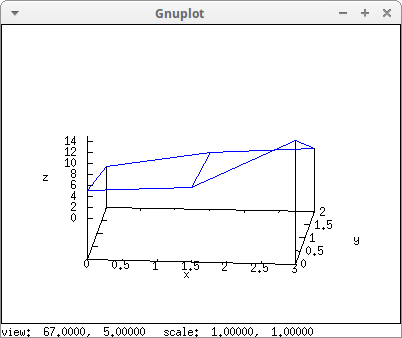
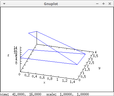
With this new object, our surfaces defined on a regular grid of the xy plane, can be expanded to a more general class, giving arbitrary values to the x and y coordinates:
draw3d(
    xlabel="x",
    ylabel="y",
    zlabel="z",
    mesh([[0,2,0],[3/2,2,3],[0,4,4]],
         [[0,0,5],[3/2,0,6],[0,2,15]])) $
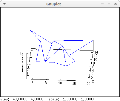
A larger mesh object:
my_grid :
  mesh([[1,1,3],[7,3,1],[12,-2,4],[15,0,5]],
       [[2,7,8],[4,3,1],[10,5,8],[12,7,1]],
       [[-2,11,10],[6,9,5],[6,15,1],[20,15,2]]) $

draw3d(my_grid)$
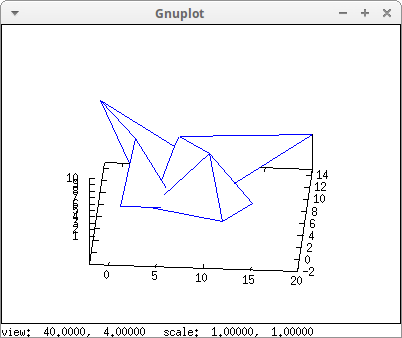
The same as above, but with hidden surfaces:
draw3d(
  surface_hide = true,
  mesh(my_grid))$
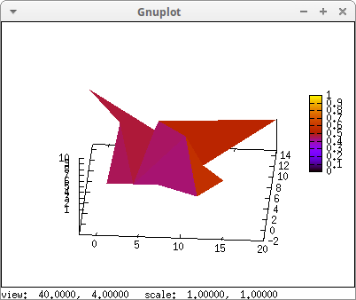
The same surface of the previous examples with enhanced3d coloring:
draw3d(
  enhanced3d = ['random(1.0),i,j],
  mesh(my_grid))$
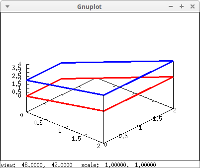
The smallest grid made by mesh is a quadrangle, at least in theory, since the four points do not need to be coplanar. Here is a multiplot with examples:
quad1 : mesh([[0,0,0], [0,1,0]],
             [[2,0,2], [2,2,2]]) $
quad2 : mesh([[0,0,2], [0,1,2]],
             [[2,0,4], [2,2,4]]) $

draw3d(
   line_width = 3,
   color      = red,
   quad1,
   color      = blue,
   quad2 ) $
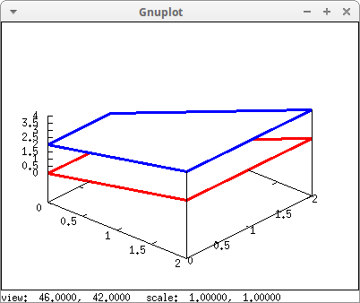
As before, but with hidden surfaces:
draw3d(
   surface_hide = true,
   line_width   = 3,
   color        = red,
   quad1,
   color        = blue,
   quad2 ) $
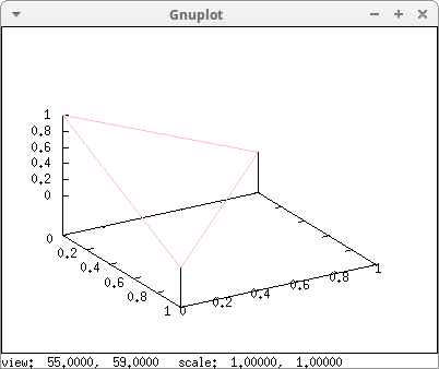
When two vertices have equal coordinates, it's a triangle:
draw3d(
  color = pink,
  mesh([[1,0,0],[0,1,0]],
       [[0,0,1],[0,0,1]]) ) $
A pyramid is built combining four triangles and one square:
options: [
   surface_hide = true,
   color        = red,
   line_width   = 3] $

triangle(p1,p2,p3) :=  mesh([p1,p2], [p3,p3]) $

quadrangle(p1,p2,p3,p4) := mesh([p1,p2], [p3,p4]) $

pyramid :
  [  triangle([1,0,0],[0,1,0],[0,0,1]),
     triangle([1,0,0],[0,-1,0],[0,0,1]),
     triangle([-1,0,0],[0,1,0],[0,0,1]),
     triangle([-1,0,0],[0,-1,0],[0,0,1]),
     quadrangle([-1,0,0],[0,1,0],[0,-1,0],[1,0,0]) ] $

draw3d(options, pyramid) $
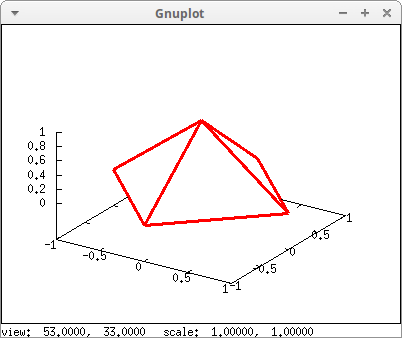
With some inspiration, we can draw the pyramid with only one mesh object
draw3d(
  mesh(
    [[0,1,0], [0,0,1], [0,0,1], [1,0,0]],
    [[0,0,1], [0,1,0], [1,0,0], [0,0,1]],
    [[0,0,1], [-1,0,0], [0,-1,0], [0,0,1]],
    [[-1,0,0], [0,0,1], [0,0,1], [0,-1,0]])  ) $

For polygons in 3D, we have to make a triangulation. Note that all quadrangles have a common vertex:
draw3d(
  surface_hide = true,
  color        = blue,
  line_width   = 3,
  mesh([[0,4,0],[4,1,0],[2,-3,0],[-2,-3,0],[-4,-1,0],[0,4,0]],
       [[0,0,0],[0,0,0], [0,0,0],[0,0,0],[0,0,0],[0,0,0]]),
  color        = red,
  mesh([[0,4,1],[4,1,1],[2,-3,1],[-2,-3,1],[-4,-1,1],[0,4,1]],
       [[0,0,1],[0,0,1], [0,0,1],[0,0,1],[0,0,1],[0,0,1]])    )$
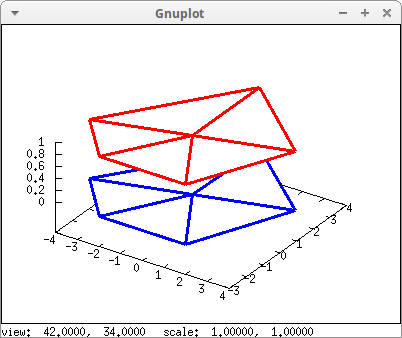
The problem is that all the triangles are visible. In order to avoid this problem, we can draw the polygon with white lines and then re-draw the perimeter with a different color.
convex_polygon(vertices, perimeter_color) :=
  block([vert : endcons(vertices[1],vertices)],
  [/* draw triangles in white */
   color = white,
   mesh(vert,
        makelist(vert[1],k,1,length(vert)) ),

   /* draw perimeter */
   points_joined = true,
   color         = perimeter_color,
   line_width    = 3,
   point_type    = dot,
   points (vert) ]) $

draw3d(
  surface_hide = true,
  convex_polygon([[0,4,0],[4,1,0],[2,-3,0],[-2,-3,0],[-4,-1,0]], blue),
  convex_polygon([[0,4,1],[4,1,1],[2,-3,1],[-2,-3,1],[-4,-1,1]], red) )$
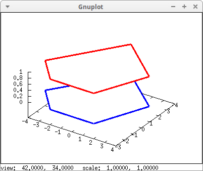
Also, with the help of the convex_polygon function defined above, we can plot other types of polyhedra:
p : %phi$

v: [[0, p, 1/p], [0, p, -1/p], [0, -p, 1/p], [0, -p, -1/p],
    [1/p, 0, p], [1/p, 0, -p], [-1/p, 0, p], [-1/p, 0, -p],
    [p, 1/p, 0], [p, -1/p, 0], [-p, 1/p, 0], [-p, -1/p, 0],
    [1, 1, 1], [1, 1, -1], [1, -1, 1], [1, -1, -1],
    [-1, 1, 1], [-1, 1, -1], [-1, -1, 1], [-1, -1, -1]]$

pentagons :
  [[v[1],v[2],v[14],v[9],v[13]],
   [v[1],v[17],v[7],v[5],v[13]],
   [v[2],v[18],v[8],v[6],v[14]],
   [v[2],v[18],v[11],v[17],v[1]],
   [v[13],v[5],v[15],v[10],v[9]],
   [v[18],v[8],v[20],v[12],v[11]],
   [v[3],v[4],v[20],v[12],v[19]],
   [v[20],v[4],v[16],v[6],v[8]],
   [v[3],v[4],v[16],v[10],v[15]],
   [v[3],v[19],v[7],v[5],v[15]],
   [v[6],v[14],v[9],v[10],v[16]],
   [v[7],v[19],v[12],v[11],v[17]]]  $

draw(
  [terminal   = animated_gif,
   dimensions = [400, 400],
   delay      = 30],
  makelist(
    gr3d(title             = "Dodecahedron",
         view              = [5 * k, 10 * k],
         proportional_axes = xyz,
         axis_3d           = false,
         surface_hide      = true,
         apply(append,makelist(convex_polygon(k,blue),k,pentagons)) ),
    k,0,36) )$
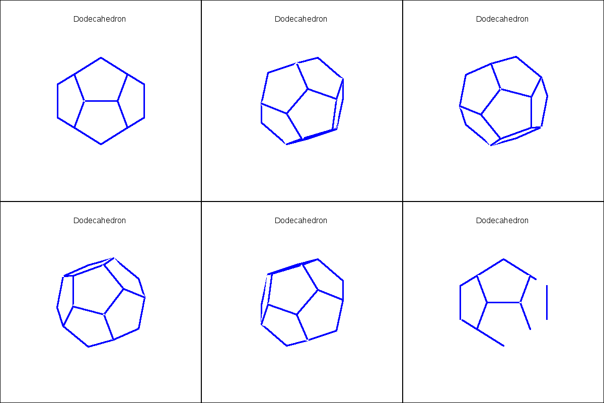
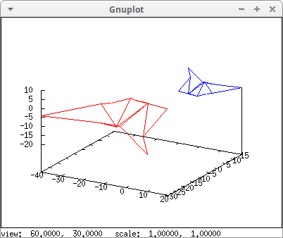
Scaling and reflecting trough the origin a mesh object:
my_grid :
  mesh([[1,1,3],[7,3,1],[12,-2,4],[15,0,5]],
       [[2,7,8],[4,3,1],[10,5,8],[12,7,1]],
       [[-2,11,10],[6,9,5],[6,15,1],[20,15,2]]) $

draw3d(
  my_grid,
  color     = red,
  transform = [-2*x,-2*y,-2*z,x,y,z],
  my_grid )$
© 2011-2016, TecnoStats.