Along this section, we are going to build interpolation curves, based on cubic splines, passing through a set of arbitrary points spread in space.
First step is to load package interpol,
load("interpol")$
Since we want to show graphical results with the VTK graphics library, let us also load package draw and set the corresponding draw renderer,
load("draw") $
draw_renderer: vtk $
Generate a set of n = 5 random points,
n: 5 $
p: makelist(makelist(random(10),2), n);
[[9,0],[9,4],[7,6],[9,9],[3,9]]
Extract the x coordinates and interpolate them by cubic splines,
cs1: cspline(map(first,p), varname=t);
(−27t328+81t228−27t14+9)charfun2(t,−∞,2)+(69t328−1035t228+2469t14−18397)charfun2(t,4,∞)+(−121t328+1245t228−2091t14+12017)charfun2(t,3,4)+(79t328−555t228+87t2−1497)charfun2(t,2,3)
Function charfun_2 returns 1 if the first argument belongs to the interval defined by the other two arguments.
Now, the same procedure with the y coordinates
cs2: cspline(map(second,p), varname=t);
(−37t356+111t256+75t28−4)charfun2(t,−∞,2)+(51t356−765t256+1887t28−7027)charfun2(t,4,∞)+(−87t356+891t256−1425t28+4027)charfun2(t,3,4)+(73t356−549t256+105t4−1387)charfun2(t,2,3)
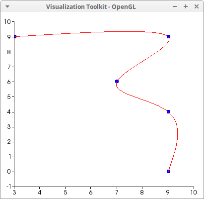
Let's plot our results,
draw2d(
  point_type = circle,
  points(p),
  nticks     = 70,
  color      = red,
  parametric(cs1,cs2, t, 1, n)) $

If we want to interpolate at t=2.5,
ev([cs1,cs2], t=2.5);
[7.665178571428569,5.006696428571427]
Just as in the 2D example, let Maxima generate n = 5 random points in the three dimensional world,
n: 5 $
p: makelist(makelist(random(10),3), n);
[[2,2,4],[5,4,1],[9,5,8],[3,5,5],[0,6,9]]
Extract the x, y, and z coordinates,
cs1: cspline(map(first,p),varname=t) $
cs2: cspline(map(second,p),varname=t) $
cs3: cspline(map(third,p),varname=t) $
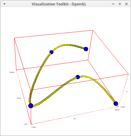
Plot the parametric curve passing through the random points,
draw3d(
  point_type = sphere,
  point_size = 0.5,
  points(p),
  line_type  = tube,
  color      = yellow,
  line_width = 0.1,
  parametric(cs1,cs2,cs3, t, 1, 5)) $

Interpolation at t=2.5,
ev([cs1,cs2,cs3], t=2.5);
[7.790178571428569,4.674107142857142,4.707589285714292]
© 2016, TecnoStats.