The following matrix has three columns, the first is the number of items my company can produce (Q), the second column are fixed costs (Cf), which are constant, and the third column are the variable costs (Cv).
d: matrix([10,75,170], [20,75,280],
          [30,75,350], [40,75,400],
          [50,75,450], [60,75,520],
          [70,75,630], [80,75,800],
          [90,75,1050],[100,75,1400]);
(1075170207528030753504075400507545060755207075630807580090751050100751400)
We can easily extract quantities and costs from the matrix,
[Q, Cf, Cv]: args(transpose(d));
[[10,20,30,40,50,60,70,80,90,100],[75,75,75,75,75,75,75,75,75,75],[170,280,350,400,450,520,630,800,1050,1400]]
Total costs are Ct=Cf+Cv,
Ct: Cf+Cv;
[245,355,425,475,525,595,705,875,1125,1475]
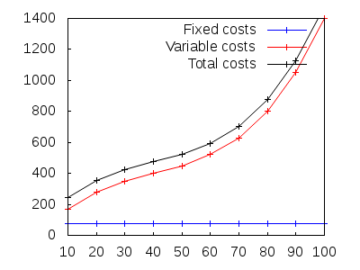
All costs in one plot,
draw2d(
  points_joined = true,
  yrange        = [0,1400],

  key           = "Fixed costs",
  points(Q, Cf),

  key           = "Variable costs",
  color         = red,
  points(Q, Cv),

  key           = "Total costs",
  color         = black,
  points(Q, Ct));

We define the average fixed cost as ¯Cf=CfQ,
Cfm: Cf/Q;
[152,154,52,158,32,54,1514,1516,56,34]
The average variable cost as ¯Cv=CvQ,
Cvm: Cv/Q;
[17,14,353,10,9,263,9,10,353,14]
And the average total cost as the sum ¯Ct=¯Cf+¯Cv,
Ctm: Cfm+Cvm;
[492,714,856,958,212,11912,14114,17516,252,594]
Also, the marginal cost is the quotient between the variation of total cost and the variation of produced units. Algebraically speaking, Cmg=ΔCtΔQ. The meaning of this concept is the additional cost of producing an additional unit of product. Let's calculate it,
Cmg: makelist((Ct[k]-Ct[k-1]) / (Q[k]-Q[k-1]),
              k, 2, length(Q)) ;
[11,7,5,5,7,11,17,25,35]
draw2d(
  points_joined = true,

  key           = "Average variable cost",
  points(Q, Cvm),

  key           = "Average total cost",
  color         = red,
  points(Q, Ctm),

  key           = "Marginal costs",
  line_width    = 2,
  color         = black,
  points(rest(Q), Cmg) )$

If my company sells each item at the price of 15€. Incomes are I=15Q,
I: 15*Q;
[150,300,450,600,750,900,1050,1200,1350,1500]
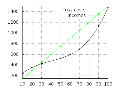
Let's make a graphical representation of both total costs and incomes against the number of items we can produce,
draw2d(
  points_joined = true,
  grid          = true,

  key           = "Total costs",
  color         = black,
  points(Q, Ct),

  key           = "Incomes",
  color         = green,
  points(Q, I) ) $

The intersection point of the two curves gives the threshold of profitability, that is, the critical number of items to be produced by my company in order to cover all costs. Any change in this production plan gives rise to profit or loss.
We want to calculate precisely this threshold point. Since we only have at hand isolated values of quantities, costs and incomes, a possible estimation is via interpolation techniques. We start loading the interpol package,
load(interpol) $
The Lagrange method of interpolation returns a polynomial that passes through all empirical points. First, for the total costs,
lct: expand(lagrange(transpose(matrix(Q,Ct)), varname=q));
q3300−2q25+62q3+75
Second, for the incomes,
lin: expand(lagrange(transpose(matrix(Q,I)), varname=q));
15q
Graphical representation of the two interpolators,
draw2d(
  grid  = true,

  color = black,
  points(Q, Ct),
  key   = "Total costs",
  explicit(lct,q,10,100),

  color = green,
  key   = "",
  points(Q, I),
  key   = "Incomes",
  explicit(lin,q,10,100) ) $

The last step is to solve equation I=Ct, but since it is a polynomial equation of fifth degree, there is not an exact algebraic method for solving it. We choose a numerical procedure instead,
find_root (lin-lct, q, 20, 30);
27.23174620148754
When the production level is below 27.23 we loss money, but for greater values, we get profit, which is the difference I−Ct. We see that the two curves have another intersection around q≈100. The maximum benefit is somewhere between these two numbers. Let's calculate the maximum of the difference I−Ct,
solve( diff(lin-lct, q));
[q=−10√93−1203,q=10√93+1203]
In decimal format,
float(%);
[q=7.854497463356816,q=72.14550253664318]
Clearly, our best decision is to produce a total amount of 72 units. The estimated benefit is
subst(q=rhs(second(%)), lin-lct);
346.4467952524305
© 2016, TecnoStats.