Empirical velocity data

The following table contains different velocity measures of a flying object, the first column corresponds to the moments of observations in seconds, and the second column to velocities in meters per second.

Let's introduce these data into Maxima and see how they look like,

table:
  [[0,0],
   [10,25],
   [15,36],
   [20,68],
   [25,93],
   [30,97],
   [35,99]]$

load(draw)$
draw2d(
  points_joined = true,
  grid          = true,
  points(table)) $

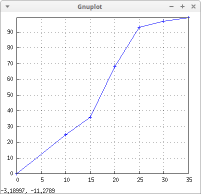
Observed data are joined by segments or linear interpolators, we can take advantage of them to estimate velocities in any point between 0 and 35 seconds.

load("interpol") $

lin: linearinterpol(table, varname=t);

$${{5\,t\,{\it charfun_2}\left(t , -\infty , 10\right)}\over{2}}+ \left({{2\,t}\over{5}}+85\right)\,{\it charfun_2}\left(t , 30 , \infty \right)+ \\ \left({{4\,t}\over{5}}+73\right)\,{\it charfun_2} \left(t , 25 , 30\right)+\left(5\,t-32\right)\,{\it charfun_2}\left( t , 20 , 25\right)+ \\ \left({{32\,t}\over{5}}-60\right)\, {\it charfun_2}\left(t , 15 , 20\right)+\left({{11\,t}\over{5}}+3 \right)\,{\it charfun_2}\left(t , 10 , 15\right)$$

In the result above, function charfun_2 is defined in package interpol and returns 1 if the first argument belongs to the interval defined by the other two arguments.

If we want an estimation of the velocity of the flying object at $t=7 s$ and $t=24 s$, we can define a function,

v1(t) := ''lin $
[v1(7), v1(24)] ;

$$\left[ {{35}\over{2}} , 88 \right]$$

In case we prefer a smooth function for interpolation, an alternative is the Lagrangian polynomial,

lag: lagrange(table, varname=t);

$${{33\,\left(t-30\right)\,\left(t-25\right)\,\left(t-20\right)\, \left(t-15\right)\,\left(t-10\right)\,t}\over{4375000}}- \\ {{97\,\left( t-35\right)\,\left(t-25\right)\,\left(t-20\right)\,\left(t-15\right) \,\left(t-10\right)\,t}\over{2250000}}+\\ {{31\,\left(t-35\right)\, \left(t-30\right)\,\left(t-20\right)\,\left(t-15\right)\,\left(t-10 \right)\,t}\over{312500}}-\\ {{17\,\left(t-35\right)\,\left(t-30\right) \,\left(t-25\right)\,\left(t-15\right)\,\left(t-10\right)\,t}\over{ 187500}}+\\ {{\left(t-35\right)\,\left(t-30\right)\,\left(t-25\right)\, \left(t-20\right)\,\left(t-10\right)\,t}\over{31250}}-\\ {{\left(t-35 \right)\,\left(t-30\right)\,\left(t-25\right)\,\left(t-20\right)\, \left(t-15\right)\,t}\over{150000}}$$

This is a sixth degree polynomial,

lag: expand(lag);

$$-{{67\,t^6}\over{39375000}}+{{92\,t^5}\over{328125}}-{{1051\,t^4 }\over{63000}}+{{2351\,t^3}\over{5250}}-{{168359\,t^2}\over{31500}}+ {{13238\,t}\over{525}}$$

We interpolate again for $t=7 s$ and $t=24 s$,

v2(t) := ''lag $
[v2(7), v2(24)] ;

$$\left[ {{2552418}\over{78125}} , {{7003392}\over{78125}} \right]$$

Let's now add the Lagrange polynomial to our plot of observed data,

draw2d(
  points_joined = true,
  grid          = true,
  points(table),
  color         = red,
  explicit (v2(t),t,0,35)) $

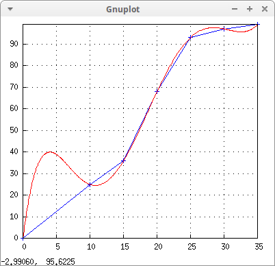
As is easily seen, the Lagrange polynomial can be a bad interpolator near the boundaries of the experimental data.

In case we want an estimation of the instantaneous acceleration in $t=17$, since $a(t)=\frac{d v(t)}{d t}$, we can differentiate the interpolator,

/* in m/s^2 */
float(subst(t=17, diff(v2(t),t)));

$$6.492423771428571$$

The mean velocity during time interval $[10,25]$, defined as $\frac{1}{25-10} \int_{10}^{25} v(t) dt$, is

/* in m/s */
float(integrate(v2(t),t, 10, 25) / (25-10));

$$53.77636054421769$$

The distance covered during this time interval is given by $\int_{10}^{25} v(t) dt$, which is equal to

/* in m */
float(integrate(v2(t),t, 10, 25));

$$806.6454081632653$$

© 2016, TecnoStats.