
Once you have opened a Maxima session, load package draw and then set global variable draw_renderer to vtk:
load("draw") $
draw_renderer: 'vtk $
To read the documentation on object explicit, write the following sentence:
describe(explicit) $
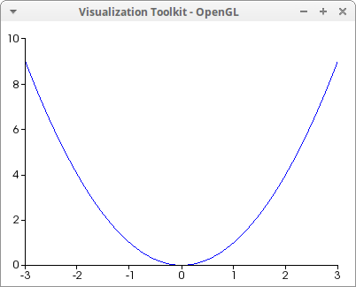
A simple plot in 2D:
draw2d(explicit(u^2,u,-3,3)) $
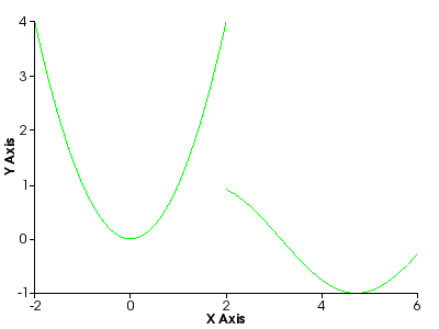
Piece-wise function exported to png:
draw2d(
    terminal   = png,
    color      = green,
    dimensions = [400,300],
    xlabel     = "X Axis",
    ylabel     = "Y Axis",
    explicit(u^2,u,-2,2),
    explicit(sin(z),z,2,6)) $
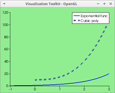
Two curves with background color and legend:
draw2d(
    background_color = light_green,
    key              = "Exponential func",
    color            = blue,
    line_width       = 2,
    explicit(exp(x),x,-1,3),
    line_width      = 5,
    line_type       = dashes,
    color           = "#4567a5",
    key             = "Cubic poly",
    explicit(%pi*x^3+sqrt(2)*x^2+10,x,0,3)) $
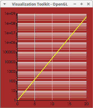
Logarithmic scale. There is a known bug here: if you don't see the curve in logarithmic scales, clic on the image to refresh it:
draw2d(
    dimensions       = [300,500],
    logy             = true,
    line_width       = 3,
    color            = yellow,
    explicit(exp(x),x,0.1,20),
    background_color = brown,
    grid             = true) $
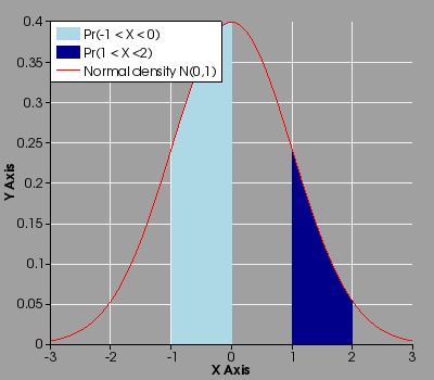
Filled function exported to PNG format:
load(distrib)$

draw2d(
    terminal         = jpg,
    dimensions       = [400,350],
    grid             = true,
    key_pos          = top_left,
    background_color = dark_grey,
    xlabel           = "X Axis",
    ylabel           = "Y Axis",

    filled_func      = true,
    fill_color       = light_blue,
    key              = "Pr(-1 < X < 0)",
    explicit(pdf_normal(x,0,1),x,-1,0),

    key              = "Pr(1 < X <2)",
    fill_color       = "dark-blue",
    explicit(pdf_normal(x,0,1),x,1,2),

    filled_func      = false,
    color            = red,
    key              = "Normal density N(0,1)",
    explicit(pdf_normal(x,0,1),x,-3,3)  ) $
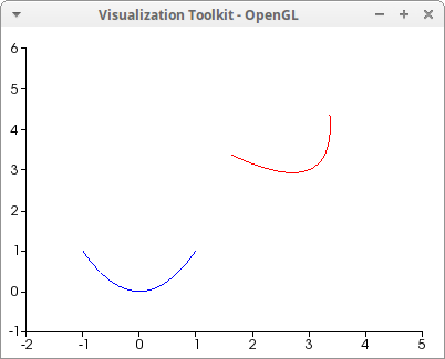
Geometric transformation of a 2d explicit curve:
th : %pi/6$

draw2d(
   xrange    = [-2,5],
   yrange    = [-1,6],

   explicit(x^2,x,-1,1),
   transform = [cos(th)*x - sin(th)*y + 3,
                sin(th)*x + cos(th)*y + 3, x, y],
   color     = red,
   explicit(x^2,x,-1,1) )$
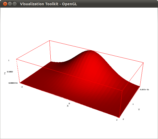
A simple red colored surface:
draw3d(
  color = red,
  explicit(exp(-x^2-y^2),x,-2,2,y,-2,0)) $
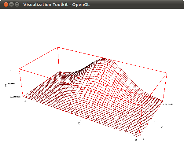
If you now press key w, you can see the wired structure of the surface:
To see the colored surface again, press now key s.
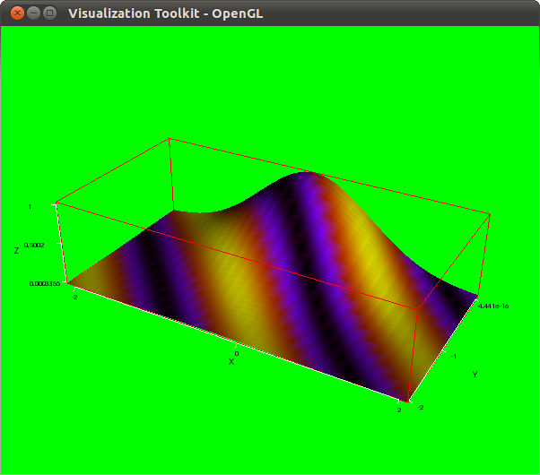
When option enhanced3d is not false, the surface is colored according to the actual palette. The behavior here is the same as in the Gnuplot case:
draw3d(
  background_color = green,
  enhanced3d       = [sin(3*(x+y)),x,y],
  explicit(exp(-x^2-y^2),x,-2,2,y,-2,0) )$
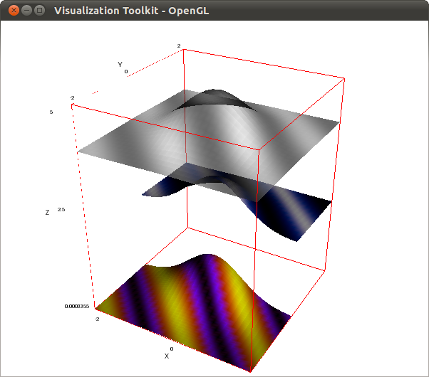
Rendering three explicit colored surfaces, each with its own palette; with VTK, option palette is a local option, which is not the case with Gnuplot, where multiple palettes are not allowed within the same scene. Also, the third surface is assigned an opacity level of 0.6; opacity is an option not available for the Gnuplot renderer:
draw3d(
  enhanced3d = [sin(3*(x+y)),x,y],
  explicit(exp(-x^2-y^2),x,-2,2,y,-2,0),

  palette = [-23, 6, -3],
  explicit(exp(-x^2-y^2)+2,x,-2,2,y,0,2),

  palette = gray,
  opacity = 0.6,
  explicit(exp(-x^2-y^2)+4,x,-2,2,y,-2,2) )$
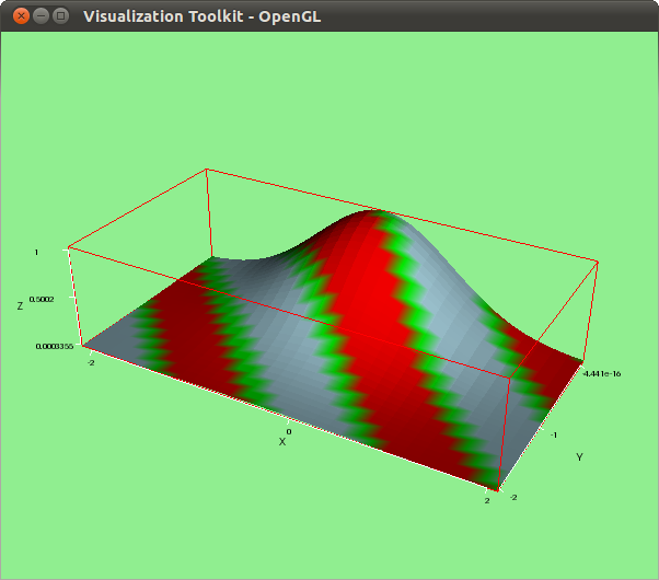
User defined palettes are also possible; in such cases, assign option palette a list of colors. The first color will be assigned to the points in the surface with the lowest level, according to enhanced3d, while the last color is assigned to the highest value, and the rest are conveniently interpolated. User defined palettes have been also incorporated for the Gnuplot renderer:
draw3d(
  background_color = light_green,
  palette          = ["#ff0000", green, light_blue],
  enhanced3d       = [sin(3*(x+y)),x,y],
  explicit(exp(-x^2-y^2),x,-2,2,y,-2,0) )$
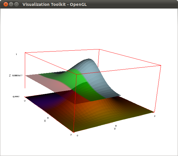
Going one step further, we can vary the opacity from one point to another if instead of a list of colors we assign option palette a list of pairs formed by the color and the opacity level. In this example, red is 50% transparent and light blue 100% opaque:
draw3d(
  palette = [["#ff0000",0.5], [green,0.8], [light_blue,1]],
  enhanced3d = y,
  explicit(exp(-x^2-y^2),x,-2,2,y,-2,0),
  palette = color,
  enhanced3d = x,
  explicit(exp(-x^2-y^2)-1,x,-2,2,y,-2,2) )$
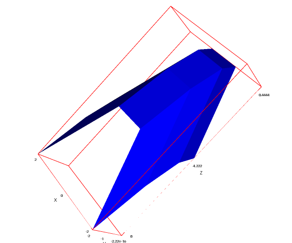
The number of points to be calculated before plotting an explicit surface can be controlled by options xu_grid and yv_grid. See also in this example that the default color is blue:
draw3d(
  xu_grid = 3,
  yv_grid = 3,
  explicit(x^2+y^2, x, -2, 2, y, -2, 0) )$
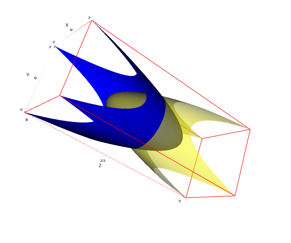
Draw's transform option is also available for explicit functions in VTK:
draw3d(
  explicit(x^2+y^2,x,-2,2,y,-2,2),
  color     = yellow,
  opacity   = 0.5,
  transform = [x, y, -z+5, x, y, z],
  explicit(x^2+y^2,x,-2,2,y,-2,2))$
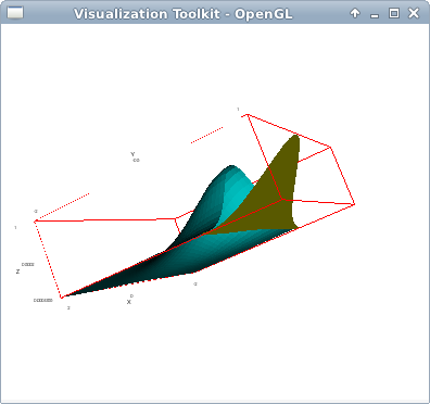
Projecting an explicit surface onto a plane:
draw3d(
  color = cyan,
  explicit(exp(-x^2-y^2),x,-2,2,y,-2,0),

  color     = yellow,
  transform = [x,z,z,  x,y,z],
  explicit(exp(-x^2-y^2),x,-2,2,y,-2,0) )$
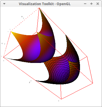
Two explicit surfaces with the same palette. In one of them, option wired_surface is set to true. In the VTK interface, option wired_surface is local, but global in the Gnuplot interface:
draw3d(
  enhanced3d    = true,
  explicit(x^2+y^2+2,x,-1,1,y,-1,1),
  wired_surface = true,
  explicit(x^2+y^2,x,-1,1,y,-1,1) ) $
Isolines of z values (default scalars) on an explicit surface:
draw3d(
  isolines   = true,
  line_width = 4,
  explicit(exp(-x^2-y^2),x,-2,2,y,-2,2))$
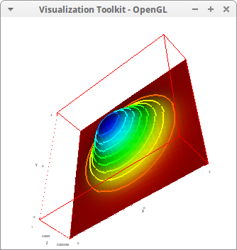
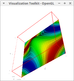
Isolines of user defined scalars. The syntax for isolines values is the same used by enhanced3d. When using the formula syntax, the names of the variables must be the same used in explicit:
draw3d(
  isolines   = sin(x*y),
  line_width = 2,
  explicit(exp(-x^2-y^2),x,-2,2,y,-2,2)) $
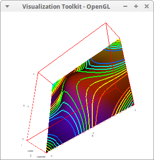
We can visualize two scalar fields playing together with isolines and enhanced3d:
draw3d(
  enhanced3d = x+y,
  isolines   = sin(x*y),
  line_width = 4,
  explicit(exp(-x^2-y^2),x,-2,2,y,-2,2)) $
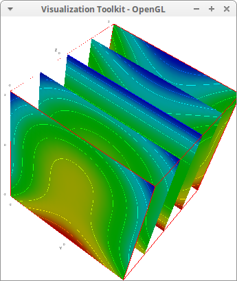
Multiple slices of a scalar field. Remember: using the list syntax, the first element is the expression of the scalar field and the rest are the names of the three coordinates, which can be arbitrary named:
draw3d(
  isolines = [2/3*x^3-y^2*z-3*z, x, y, z],
  makelist(explicit(k,x,-2,2,y,-2,2), k, -2, 2))$
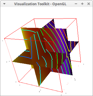
Orthogonal slices. The surfaces are colored according to scalar field F(x,y,z)=2/3*x^3-y^2*z-3*z, but isolines are plotted according to a translation of F(x,y,z):
draw3d(
    enhanced3d=[2/3*x^3-y^2*z-3*z, x, y, z],

    isolines = [2/3*(x-2)^3-(y+3)^2*(z+1)-3*(z+1), x, y, z],
    line_width=4,

    /* XY-plane */
    explicit(0,x,-2,2,y,-2,2),

    /* YZ-plane */
    transform = [z,x,y+z,x,y,z],
    explicit(0,x,-2,2,y,-2,2),

    /* XZ-plane */
    transform = [x,-z,y,x,y,z],
    explicit(0,x,-2,2,y,-2,2) )$
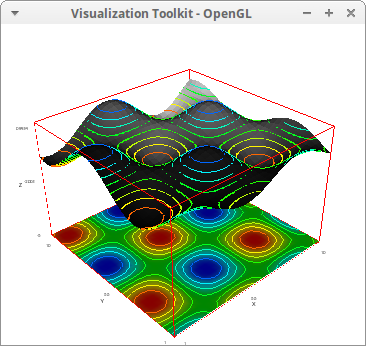
Isolines of an explicit surface are projected onto a plane:
draw3d(
  line_width = 2,
  enhanced3d = [x*y,x,y],
  palette    = gray,
  isolines   = true,
  explicit(sin(x)*cos(y),x,1,10,y,1,10),

  /* isolines projected on the plane */
  enhanced3d    = false,
  isolines      = [sin(x)*cos(y),x,y],
  explicit(-5,x,1,10,y,1,10)  ) $
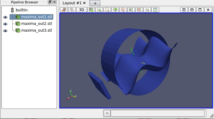
Setting terminal=stl, Maxima creates a 3D scene in stl format. In this example, file maxima_out.stl is generated, which is later explored with Paraview. Note that colors are lost in format stl:
draw3d(
  terminal = stl,
  cylinder([0,0,0],5,5,[0,1,0]),
  color    = orange,
  cube(1/2, 5, 3, [7, 0, 0]),
  color    = white,
  explicit(sin(x)+cos(y), x,-5,5,y,-5,5)) $
Also, we can explore the stl scene with the javascript magic of Three (rotate with left button, zoom in and out with right button, change position with wheel button):
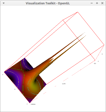
Make use of zrange option in the presence of poles:
draw3d(
  zrange     = [-10,15],
  enhanced3d = [sin(x)+cos(y),x,y],
  isolines   = [sin(x)+cos(y),x,y],
  explicit(1/(x^2+y^2), x, -3, 3, y, -3, 3)) $
Another use of zrange:
draw3d(
  zrange = [-5,5],
  explicit(x^2+y^2, x, -1, 1, y, -1, 1),
  color  = red,
  explicit(1/(x+y), x, -2, 2, y, -2, 2)) $
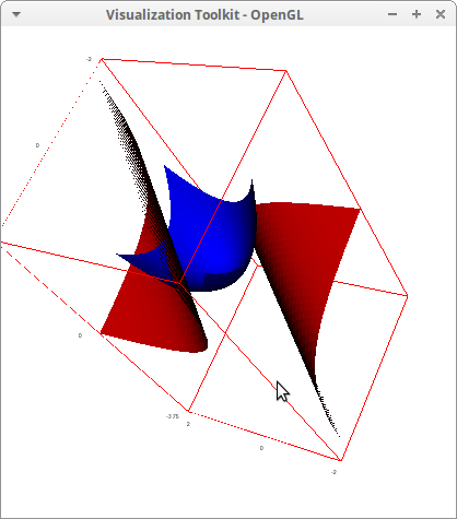
Isolines from 0.25 to 0.7 is steps of 0.05:
draw3d(
  isolines_levels = [0.25,0.05,0.7],
  isolines        = true,
  explicit(10*exp(-x^2-y^2), x, -2, 2, y, -2, 2)) $
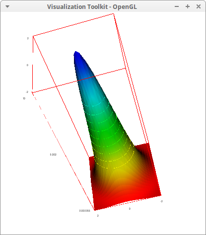
Generate 10 equal spaced isolines:
draw3d(
  isolines_levels = 10,
  isolines        = [x,x,y,z],
  explicit(10*exp(-x^2-y^2), x, -2, 2, y, -2, 2)) $
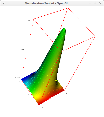
Isolines at user defined levels:
draw3d(
  isolines_levels = {0.2,0.4,0.8},
  isolines        = [cos(x+y),x,y],
  explicit(3*exp(-x^2-y^2), x, -2, 2, y, -2, 2)) $
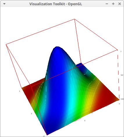
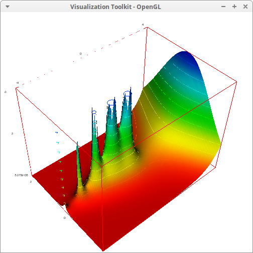
Complex valued gamma function, Γ(z)=∫∞0xz−1e−xdx:
draw3d(
  zrange          = [0,6],
  xu_grid         = 100,
  yv_grid         = 100,
  isolines        = true,
  isolines_levels = [0,0.1,6],
  explicit(cabs(gamma(x+%i*y)),x,-4,4,y,-3,3)) $
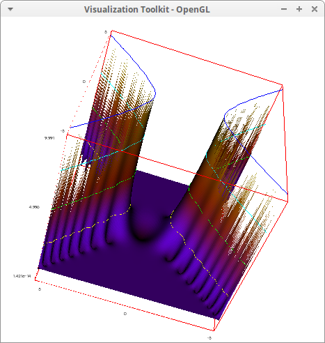
Complex valued error function, erf(z)=2√π∫z0xz−1e−t2dt:
draw3d(
  zrange     = [-10,10],
  enhanced3d = [z,x,y,z],
  xu_grid    = 200,
  yv_grid    = 200,
  isolines   = true,
  explicit(cabs(erf(x+y*%i)), x, -5, 5, y, -5, 5) ) $
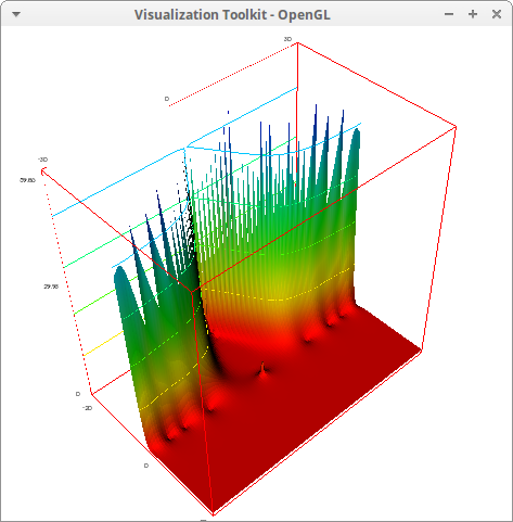
Complex valued Riemann's zeta function, ζ(z)=∑∞n=1n−z:
draw3d(
  zrange          = [0,60],
  xu_grid         = 100,
  yv_grid         = 100,
  isolines        = true,
  isolines_levels = [0,0.2,6],
  explicit(cabs(zeta(x+%i*y)),x,-20,20,y,-30,30)) $
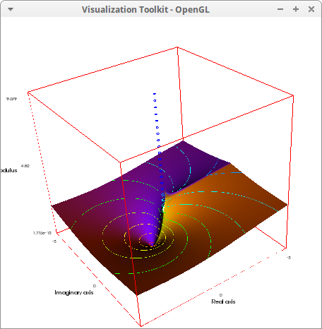
Complex valued logaritmm, log(z):
draw3d(
  enhanced3d      = [carg(log(x+y*%i)),x,y],
  xlabel          = "Real axis",
  ylabel          = "Imaginary axis",
  zlabel          = "Modulus",
  xu_grid         = 100,
  yv_grid         = 100,
  isolines_levels = [-5,0.1,5],
  zrange          = [-10,10],
  isolines        = true,
  explicit(cabs(log(x+y*%i)), x, -5, 5, y, -5, 5) ) $
© 2011-2017, TecnoStats.