Back to draw-VTK

'draw'-VTK interface:
object parametric

• Parametric functions in R²
• Parametric functions in R³

Once you have opened a Maxima session, load package draw and then set global variable draw_renderer to vtk:

load("draw") $
draw_renderer: 'vtk $

To read the documentation on object parametric, write the following sentence:

describe(parametric) $

Parametric functions in R²

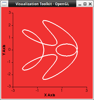
Parametric plot in 2D:

draw2d(
    background_color = light_red,
    color            = white,
    nticks           = 150,
    line_width       = 3,
    dimensions       = [300, 300],
    xlabel           = "X Axis",
    ylabel           = "Y Axis",
    parametric(
      1.5*cos(t)-cos(5*t),
      1.5*sin(t)-sin(4*t),
      t, 0, 2*%pi) )$

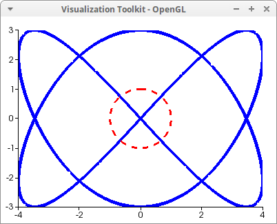
A Lisajous curve and a circumference, with different widths, colors and styles:

[a, b]: [1, 3/2] $

draw2d(
    nticks     = 200,
    line_width = 5,
    parametric(4*sin(a*t/b),3*sin(t), t, -3*%pi, 3*%pi),
    color      = red,
    line_width = 3,
    line_type  = dashes,
    parametric(sin(t),cos(t), t, 0, 2*%pi) )$

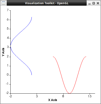
Geometric transformation of a 2d parametric curve:

para : parametric(2*cos(r),r,r,0,2*%pi) $

draw2d(
   para,
   transform = [v+6,u,u,v],
   color     = red,
   xlabel    = "X Axis",
   ylabel    = "Y Axis",
   para)$

Parametric functions in R³

A simple parametric curve:

draw3d(
  parametric(t, t, t^2, t,0 , 1) ) $

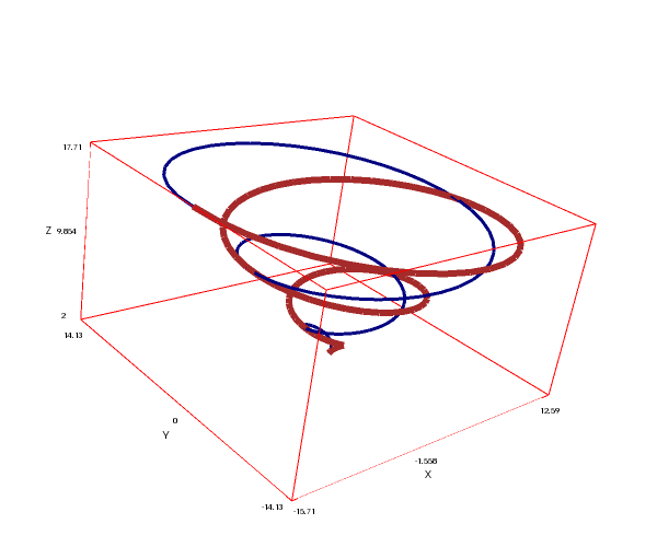
Two parametric curves of different colors and widths:

draw3d(
  nticks     = 100, 

  color      = navy,
  line_width = 3.4,
  parametric(t*cos(t),t*sin(t),2+t,t,0,5*%pi),

  color      = brown,
  line_width = 5.7,
  parametric(t*cos(t),-t*sin(t),2+t,t,0,5*%pi) )$

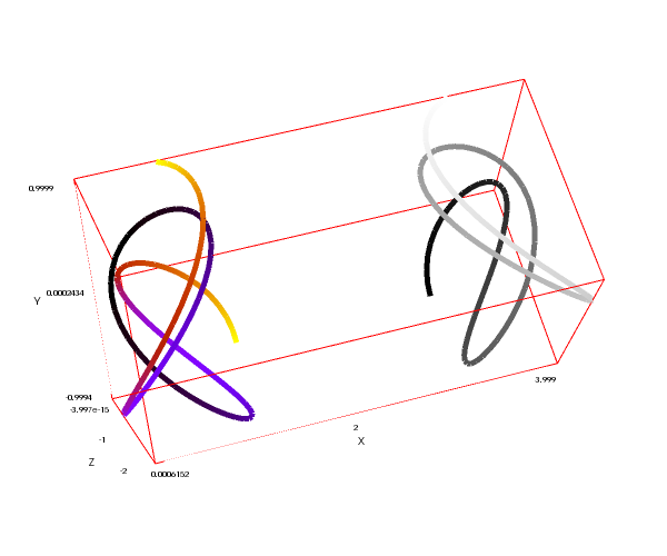
Two parametric curves with varying colors according to the enhanced3d model. Note that the curves are colored with different palettes:

draw3d(
   nticks     = 100,
   line_width = 5,

   enhanced3d = (u-1)^2,
   parametric(cos(5*u)^2,sin(7*u),u-2,u,0,2),

   palette    = gray,
   enhanced3d = [z,x,y,z],
   parametric(3+sin(5*u)^2,sin(7*u),u-2,u,0,2) ) $

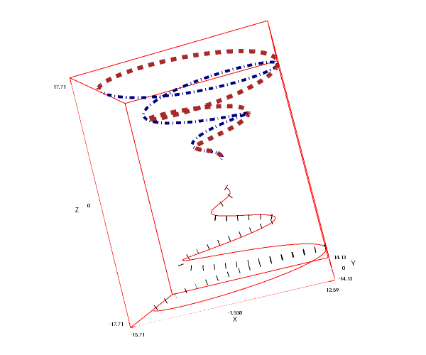
Parametric curves with different values for option line_type:

draw3d(
  nticks     = 100,

  line_type  = dot_dash,
  color      = navy,
  line_width = 4,
  parametric(t*cos(t),t*sin(t),2+t,t,0,5*%pi),

  line_type  = dashes,
  color      = brown,
  line_width = 5.7,
  parametric(t*cos(t),-t*sin(t),2+t,t,0,5*%pi),

  line_type  = solid,
  color      = red,
  line_width = 1,
  parametric(t*cos(t),-t*sin(t),-2-t,t,0,5*%pi),

  line_type = dots,
  color     = black,
  line_width = 8,
  parametric(t*cos(t),t*sin(t),-2-t,t,0,5*%pi) )$

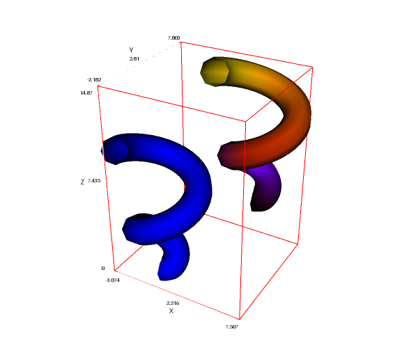
Tubular parametric curves. The first curve is painted with the default solid color, and the second with the enhanced3d model. See also that the second curve is obtained after a geometric translation:

draw3d(
  nticks     = 100,

  line_type  = tube,
  parametric(t*cos(t^2),t*sin(t^2),t^2,t,0,%pi),

  enhanced3d = true,
  transform  = [x+5, y+5, z+5, x, y, z],
  parametric(t*cos(t^2),t*sin(t^2),t^2,t,0,%pi) ) $

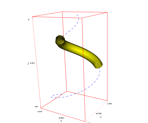
Combining a tube with dashed curve:

draw3d(
  nticks     = 100,

  line_type  = dashes,
  parametric(t*cos(t^2),t*sin(t^2),t^2,t,0,%pi),

  color      = yellow,
  line_type  = tube,
  line_width = 0.5,
  parametric(t*cos(t^2),t*sin(t^2),t^2,t, %pi/2, 3*%pi/4)) $

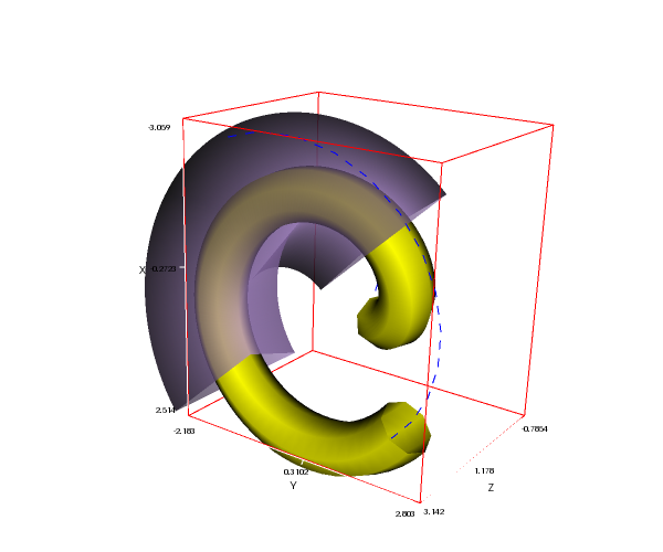
Tubes with different number of faces (minimum is three). Option opacity is also available for parametric object:

draw3d(
  nticks     = 100,
  line_type  = dashes,
  parametric(t*cos(t^2),t*sin(t^2),t,t,-%pi/4,%pi),

  color = yellow,
  line_type  = tube,
  line_width = 0.5,
  parametric(t*cos(t^2),t*sin(t^2),t,t, %pi/4, 6*%pi/7),

  color      = "#c59af0",
  line_type  = [tube, 3],
  line_width = 1.5,
  opacity    = 0.7,
  parametric(t*cos(t^2),t*sin(t^2),t,t, %pi/2, 3*%pi/4)) $

© 2011-2016, TecnoStats.