Once you have opened a Maxima session, load package draw and then set global variable draw_renderer to vtk:
load("draw") $
draw_renderer: 'vtk $
To read the documentation on object points, write the following sentence:
describe(points) $
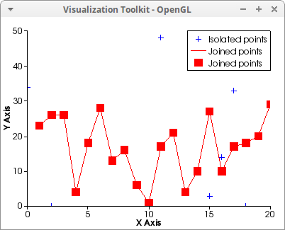
Isolated and joined points on the plane:
draw2d(
    dimensions    = [400, 300],

    key           = "Isolated points",
    points(makelist([random(20),random(50)],k,1,10)),

    point_type    = square,
    point_size    = 5,
    points_joined = true,
    color         = red,
    key           = "Joined points",
    points(makelist(k,k,1,20),makelist(random(30),k,1,20)))$
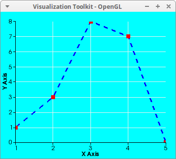
Points and segments with different colors. No legend:
pts: [[1,1],[2,3],[3,8],[4,7],[5,0]] $

draw2d(
    background_color = cyan,
    grid             = true,

    points_joined    = true,
    point_type       = square,
    line_type        = dashes,
    line_width       = 3,
    points(pts),

    color            = red,
    points_joined    = false,
    points(pts) ) $
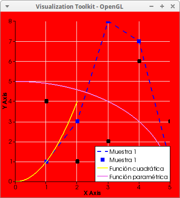
Two set of points, together with explicit and parametric curves. Note that the black isolated points are not referenced in the legend. Also, the two set of points are defined via row matrices:
draw2d(
    background_color = red,
    grid             = true,

    point_type       = square,
    line_width       = 2,
    line_type        = dashes,
    points_joined    = true,
    key              = "Muestra 1",
    points(transpose(matrix([1,3,8,7,1]))),

    point_type       = circle,
    points_joined    = false,
    color            = black,
    point_size       = 4,
    key              = "",
    points(transpose(matrix([4,1,2,6,3]))),

    color            = yellow,
    line_type        = solid,
    key              = "Función cuadrática",
    explicit(x^2,x,0,2),

    color            = violet,
    key              = "Función paramétrica",
    parametric(5*cos(t),5*sin(t), t, 0, %pi/2),

    key_pos          = bottom_right )$
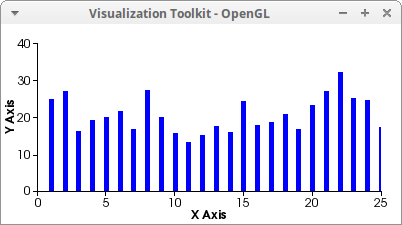
Impulses. Simulation of 25 samples of the normal distribution:
load("distrib")$

draw2d(
    points_joined = impulses,
    line_width    = 5,
    point_type    = dot,
    dimensions    = [400,200],
    points(random_normal(20,5,25)))$
Plane transformations:
/* set defaults to avoid writing them many times */
set_draw_defaults(
  points_joined = true,
  point_type = dot,
  proportional_axes = 'xy) $

/* builds a grid */
malla(x0,x1,y0,y1) :=
  block([dx, dy, n:21],
    dx: (x1-x0)/n,
    dy: (y1-y0)/n,
    append(
       makelist(
          points(makelist([x0+j*dx, y0+k*dy],
                          k, 1, n)),
          j, 1, n),
       makelist(
          points(makelist([x0+j*dx, y0+k*dy],
                          j, 1, n)),
          k, 1, n)) )$

/* an auxiliary function */
module(x,y) := sqrt(x^2+y^2) $

/* draw a non-transformed grid */
draw2d(malla(-%pi,%pi,-%pi,%pi)) $
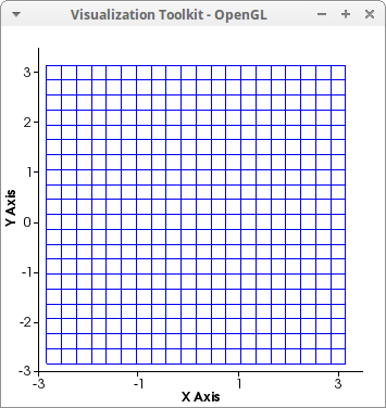
Now we apply a set of transformations to the regular grid:
tr1 :
  block([k : sin(x)*sin(y)/module(x,y)],
    gr2d(transform = [k*x+x, k*y+y, x, y],
         malla(-%pi,%pi,-%pi,%pi) )) $

tr2 :
  block([k : 1.25/(module(x,y)+0.8)/module(x,y) ],
    gr2d(transform = [k*x+x, k*y+y, x, y],
         malla(-3/2,3/2,-3/2,3/2) )) $

tr3 :
  block([k : sin(module(x,y))/module(x,y) ],
    gr2d(transform = [k*x+x, k*y+y, x, y],
         malla(-3*%pi,3*%pi,-3*%pi,3*%pi) )) $

tr4 :
  gr2d(transform = [realpart(cos(x+y*%i)),
                    imagpart(cos(x+y*%i)),
                    x, y],
       malla(-%pi, %pi, -%pi, %pi) ) $

tr5 :
  gr2d(transform = [realpart(1/conjugate(x+y*%i)),
                    imagpart(1/conjugate(x+y*%i)),
                    x, y],
       malla(-3, 3, -3, 3) ) $

tr6 :
  block([k : sin(module(x,y))],
    gr2d(transform = [k*x, k*y, x, y],
         malla(-2*%pi, 2*%pi, -2*%pi, 2*%pi) )) $

tr7 :
  block([k : sin(x*y)],
    gr2d(transform = [k*x, k*y, x, y],
         malla(-2*%pi, 2*%pi, -2*%pi, 2*%pi) )) $

tr8 :
  gr2d(transform = [y, cos(x*y), x, y],
       malla(0, %pi, 0, 2*%pi ) ) $

draw(
  columns  = 2,
  dimensions = [800,400],
  tr1, tr2, tr3, tr4, tr5, tr6, tr7, tr8 ) $

Draw 3D sample points. Valid values for point_type are: dot, plus, multiply, asterisk, square, fille_square, sphere, cube, cylinder, and cone:
/* read multivariate data from descriptive package */
s2 : read_matrix (file_search ("wind.data"))$

draw3d(
  point_size = 1/2,
  color      = red,
  point_type = multiply,
  points(args(submatrix (s2, 4, 5))) )$

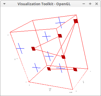
Isolated and connected points. Note that the point_size, which defaults to 1, the radius of the symbol, is an absolute measure in terms of the axes scales:
draw3d(
  /* points with default settings */
  points([[2,1,6], [-2,3,5], [3,-1,-2], [1,2,3], [-2,5,0], [0,0,0]]),

  /* another set of points */
  color         = red,
  points_joined = true,
  point_type    = filled_square,
  point_size    = 1/3,
  points([[5,1,6], [1,3,5], [6,-1,-2], [4,2,3], [1,5,0], [3,0,0]]))$
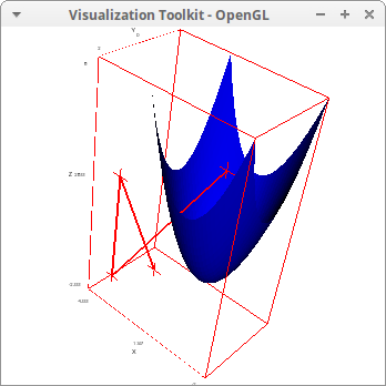
Discrete data and explicit surface:
draw3d(
  points_joined = true,
  color         = red,
  line_width    = 2,
  point_size    = 1/3,
  points([[1,2,1], [3,2,4], [4,1,-2], [0,0,5]]),

  color         = blue,
  explicit(x^2+y^2, x,-2,2,y,-2,2)) $
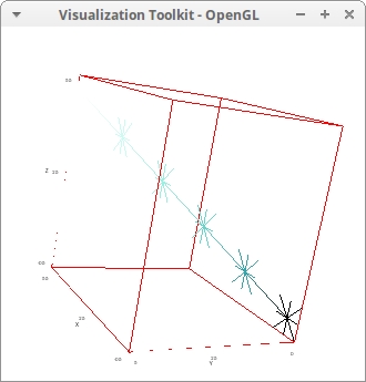
Coloring points with palette and enhanced3d model:
draw3d(
  point_size    = 1/2,
  point_type    = 3,
  palette       = [-4,-9,7],
  enhanced3d    = [sqrt(k),k], /* here, k is the order index in the points object */
  points_joined = true,
  points([[0,0,0], [1,1,1], [2,2,2], [3,3,3], [4,4,4], [5,5,5]]))$
Exporting the scene to Postscript and exploring it with the evince viewer:
draw3d(
  file_name  = "data",
  terminal   = eps,
  point_size = 1/2,
  point_type = filled_square,
  points([[3,1,6], [-1,3,5], [4,-1,-2],
          [2,2,3], [-1,5,0], [1,0,0]]))$
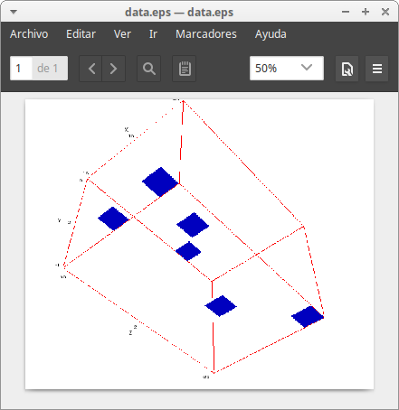
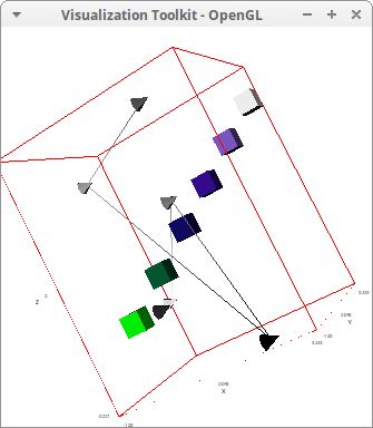
Two samples with solid glyphs (in vtk's parlance):
draw3d(
  point_size    = 1/2,
  point_type    = cone,
  palette       = gray,
  enhanced3d    = [y,x,y,z],
  points_joined = true,
  points([[3,1,6], [-1,3,5], [4,-1,-2], [2,2,3], [-1,5,0], [1,0,0]]),

  point_size    = 2/3,
  point_type    = cube,
  palette       = [5,12,-3],
  points_joined = false,
  points([[0,0,0], [1,1,1], [2,2,2], [3,3,3], [4,4,4], [5,5,5]]) )$
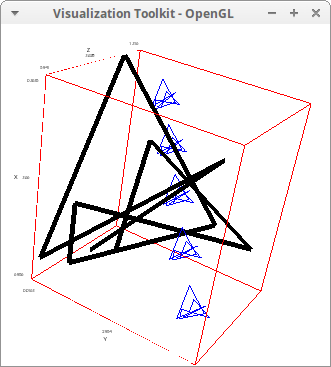
Geometric transformations in 3d points:
xyz: makelist([random(1.0), random(1.0), random(1.0)], 10)$

draw3d(
   points_joined = true,
   point_type    = dot,

   makelist(
        [transform = [x+j,y+j,z+j,x,y,z],
         points(xyz)], j, 5),

   color      = black,
   line_width = 5,
   transform  = [7*x,7*y,7*z,x,y,z],
   points(xyz) ) $
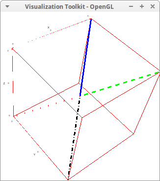
Joining points with different line types:
draw3d(
  line_width    = 3,
  points_joined = true,
  point_type    = dot,

  line_type = solid,
  color     = blue,
  points([[0,0,0], [5,5,5]]),

  line_type = dots,
  color     = red,
  points([[0,0,0], [-5,5,-5]]),

  line_type = dashes,
  color     = green,
  points([[0,0,0], [5,-5,5]]),

  line_type = dot_dash,
  color     = black,
  points([[0,0,0], [-5,-5,-5]]))$
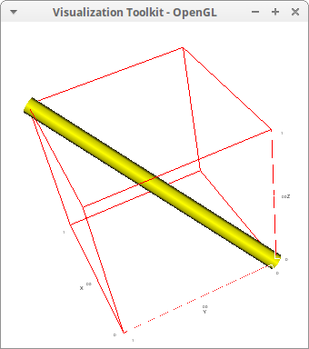
Joining two points with a tube painted with a solid color:
draw3d(
  points_joined = true,
  point_type    = dot,
  color         = yellow,
  line_width    = 0.05,
  line_type     = tube,
  points([[0,0,0], [1,1,1]])) $
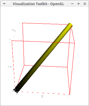
Joining two points with a tube painted with the enhanced3d model and default palette:
draw3d(
  points_joined = true,
  point_type    = dot,
  enhanced3d    = true,
  line_width    = 0.05,
  line_type     = tube,
  points([[0,0,0], [1,1,1]])) $
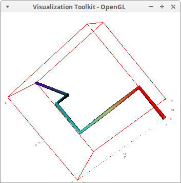
Joining a series of points with a tube painted with the enhanced3d model and a selected palette:
draw3d(
  points_joined = true,
  point_type    = dot,
  enhanced3d    = [z,x,y,z],
  line_width    = 0.05,
  line_type     = tube,
  palette       = [33, -13, 10],
  points([[0,0,0], [1,1,1],[2,1,1],[2,2,1],[2,2,2],[2,2,3],[2,3,3]])) $
The colors of my football team:
draw3d(
  points_joined = true,
  point_type    = dot,
  enhanced3d    = true,
  line_width    = 1/2,
  line_type     = tube,
  palette       = [white, blue, white, blue, white, blue],
  points([[0,0,0], [1,1,1],[2,2,2], [3,3,3], [4,4,4], [5,5,5]])) $

When option points_joined is set to impulses, vertical lines are drawn from each point to plane z=0:
s2 : read_matrix (file_search ("wind.data"))$

draw3d(
  point_size    = 1/2,
  point_type    = cube,
  enhanced3d    = [y,x,y,z],
  palette       = [5,12,-3],
  points_joined = impulses,
  color         = red, /* for vertical segments */
  points(args(submatrix (s2, 4, 5))) )$

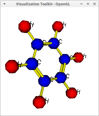
Benzene C6H6:
s: 5*sqrt(3)/2 $
v: 5*sqrt(3) $
draw3d(
   axis_3d       = false,
   point_size    = 0,
   color         = yellow,
   points_joined = true,
   line_width    = 0.3,
   line_type     = tube,
   points([[0,10,0],[0,5,0],[s,5/2,0],[v,5,0]]),
   points([[v,-5,0],[s,-5/2,0],[0,-5,0],[0,-10,0]]),
   points([[-v,5,0],[-s,5/2,0],[-s,-5/2,0],[-v,-5,0]]),
   points([[0,5,1/2],[-s,5/2,1/2]]),
   points([[0,5,-1/2],[-s,5/2,-1/2]]),
   points([[-s,-5/2,1/2],[0,-5,1/2]]),
   points([[-s,-5/2,-1/2],[0,-5,-1/2]]),
   points([[s,5/2,1/2],[s,-5/2,1/2]]),
   points([[s,5/2,-1/2],[s,-5/2,-1/2]]),
   points_joined = false,

   /* Hydrogen */
   color = red,
   point_type = sphere,
   point_size    = 3,
   points([[0,10,0], [0,-10,0], [v,5,0], [v,-5,0],
           [-v,5,0], [-v,-5,0]]),
   font_size = 1,
   color = black,
   label(["H",0,10,1.7],["H",0,-10,1.7],
         ["H",v,5,1.7],["H",v,-5,1.7],
         ["H",-v,5,1.7],["H",-v,-5,1.7]),

   /* Carbon */
   color = blue,
   points([[0,5,0], [0,-5,0], [s,5/2,0], [s,-5/2,0],
           [-s,5/2,0], [-s,-5/2,0]]),
   color = black,
   label(["C",0,5,1.7],["C",0,-5,1.7],
         ["C",s,5/2,1.7],["C",s,-5/2,1.7],
         ["C",-s,5/2,1.7],["C",-s,-5/2,1.7]) )$
© 2011-2016, TecnoStats.