Once you have opened a Maxima session, load package picture:
load("picture") $
To read the documentation on object image, write the following sentence:
describe(image) $
Package picture gives Maxima very (VERY) basic support for image processing. It's automatically loaded together with package draw. At this moment, it contains the following functions: make_level_picture, picturep, make_rgb_picture, take_channel, picture_equalp, negative_picture, rgb2level and read_xpm.
A matrix of numbers can be interpreted as a gray or color image, depending on the palette option:
im: apply('matrix,
          makelist(makelist(random(200),i,1,30),i,1,30))$
draw2d(image(im,0,0,30,30))$

draw2d(palette = gray,
       image(im,0,0,30,30))$

draw2d(palette = [15,20,-4],
       image(im,0,0,30,30))$

The same image in different positions and dimensions:
im: apply('matrix,
           makelist(makelist(random(200),i,1,30),i,1,30))$
draw2d(image(im,0,0,10,10),
       image(im,10,10,15,15),
       image(im,25,25,20,20))$

A matrix of numeric vectors of length three can be interpreted as an rgb color image:
rgb: apply('matrix,
           makelist(
             makelist(
               [random(300),random(300),random(300)],i,1,30),i,1,30))$
draw2d(image(rgb,0,0,30,30))$

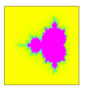
The Mandelbrot set. This program makes use of package fractals; it's not very fast, but it covers our needs for this demonstration:
load(fractals)$

make_mandelbrot(x0,y0,width,height,ncols,nrows):=
  block([dx,dy,x,y,m],
    dx: width/(ncols-1),
    dy: height/(nrows-1),
    x: makelist(x0+(i-1)*dx,i,1,ncols),
    y: makelist(y0+height-(j-1)*dy,j,1,nrows),
    m: makelist(makelist(mandelbrot_set(x[i],y[j]),
                         i,1,ncols),
                j,1,nrows),
    apply(matrix,m) )$

m:make_mandelbrot(-2.5,-1.5,3.5,3,200,200)$

mb(colors,file):=
  draw2d(
    file_name  = file,
    terminal   = png,
    dimensions = [300,300],
    xtics      = none,
    ytics      = none,
    colorbox   = false,
    palette    = colors,
    image(m, -2.5,-1.5,3.5,3))$
mb(color,"mandelbrot1")$
mb([-14,-21,30],"mandelbrot2")$
mb([1,9,-10],"mandelbrot3")$
mb(gray,"mandelbrot4")$


Let's make use of function read_xpm to read an image in XPM format and render it with Maxima. This image has been transformed from PNG to XPM with program Gimp. The XPM format is also used by Maxima in the dynamics package:
This image has dimensions 219x148. Be patient with larger ones.
cats: read_xpm("gatos.xpm")$
draw2d(image(cats,0,0,10,7))$

It's possible to combine images with any other graphic objects:
cats: read_xpm("gatos.xpm")$

draw2d(
  yrange      = [-4,10],
  ellipse(5,3,8,6,0,360),
  image(cats,0,0,10,7),
  line_width  = 2,
  head_length = 0.3,
  color       = blue,
  label(["This is Francisco",-1,-0.5]),
  vector([-1,0],[2,4]),
  color       = green,
  vector([11,7],[-2,-1]),
  label(["This is Manolita",11,8]),
  explicit(sin(x)-2,x,-4,15) )$

Once we have the original picture, there are some simple transformations to play with :
cats: read_xpm("gatos.xpm")$
negcats:  negative_picture(cats)$

draw2d(
  title = "Negative cats",
  image(negcats,0,10,10,10))$

greycats: rgb2level(cats)$

/* By default, level images are rendered with a color palette*/
draw2d(
  title = "Psychedelic cats",
  image(greycats,0,10,10,10))$

draw2d(title="True gray picture",
       palette = gray,
       image(greycats,0,10,10,10))$

Let's now take some (x,y) coordinates from a picture and compute a cubic spline interpolator. First, we save the coordinates of middle-mouse clicks (by pressing key x after clicking) in file points.txt, and then a Maxima script reads the file and computes the parametric cubic splines:
/* Saving coordinates */
draw2d(
  xy_file = "points.txt",
  image(read_xpm("Janthina_janthina.xpm"),0,0,10,10))$

This is now the contents of file points.txt:
2.00161637931034 6.06501057082452
2.20366379310345 5.95137420718816
2.16056034482759 5.70031712473573
1.82112068965517 5.6553911205074
1.66217672413793 5.97515856236786
1.79956896551724 6.40856236786469
2.36260775862069 6.6384778012685
2.8582974137931 6.40856236786469
3.06303879310345 6.02008456659619
3.10883620689655 5.6316067653277
2.99568965517241 5.19556025369979
2.63469827586207 4.83086680761099
2.04741379310345 4.62473572938689
1.39278017241379 4.96828752642706
1.03178879310345 5.74524312896406
1.25808189655172 6.70718816067653
1.79956896551724 7.34672304439746
2.79094827586207 7.78276955602537
4.01131465517241 7.66913319238901
4.82219827586207 7.09566596194503
5.25053879310345 6.33985200845666
5.47683189655172 5.31183932346723
5.34213362068966 4.41860465116279
4.80064655172414 3.48044397463002
3.89816810344828 2.86205073995772
2.8582974137931 2.65591966173362
1.86691810344828 2.93076109936575
1.07758620689655 3.43551797040169
0.557650862068966 4.41860465116279
0.355603448275862 5.56289640591966
0.738146551724138 7.16437632135307
1.8426724137931 8.55972515856237
4.12176724137931 9.65909090909091
6.42510775862069 9.33932346723044
8.00377155172414 8.40116279069768
8.54525862068965 7.8514799154334
9.06519396551724 7.07188160676533
9.38038793103448 6.08879492600423
9.56088362068965 4.28118393234672
The following code reads points.txt and computes the parametric interpolation. Results are then plotted.
load(numericalio)$
load(interpol)$

mat: read_matrix("points.txt")$
[x, y]: args(transpose(mat))$
param: makelist(t,t,1,length(mat))$
x_pairs: transpose(matrix(param,x))$
y_pairs: transpose(matrix(param,y))$
x_cspline:cspline(x_pairs, varname='t)$
y_cspline:cspline(y_pairs, varname='t)$
xx(t):= ''x_cspline$
yy(t):= ''y_cspline$

draw2d(
  title      = "Parametric cubic splines",
  image(read_xpm("Janthina_janthina.xpm"),0,0,10,10),
  nticks     = 100,
  line_width = 5,
  color      = yellow,
  parametric(xx(t),yy(t),t,1,length(mat)))$

© 2011-2016, TecnoStats.